
PostGIS Quickstart
PostGIS adds spatial capabilities to the PostgreSQL relational database. It extends PostgreSQL so it can store, query, and manipulate spatial data. In this Quickstart we will use ‘PostgreSQL’ when describing general database functions, and ‘PostGIS’ when describing the additional spatial functionality provided by PostGIS.
This Quick Start describes how to:
- Create and query a spatial database from the command line and QGIS graphical client.
- Manage data from the
pgAdminclient.
Contents
Client-server Architecture
PostgreSQL, like many databases, works as a server in a client-server system. The client makes a request to the server and gets back a response. This is the same way that the internet works - your browser is a client and a web server sends back the web page. With PostgreSQL the requests are in the SQL language and the response is usually a table of data from the database.
There is nothing to stop the server being on the same computer as the client, and this enables you to use PostgreSQL on a single machine. Your client connects to the server via the internal ‘loopback’ network connection, and is not visible to other computers unless you configure it to be so.
Creating A Spatially-Enabled database
Command-line clients run from within a Terminal Emulator window. Start a Terminal Emulator (LXTerminal currently) from the Applications menu in the Accessories section. This gives you a Unix shell command prompt. Type:
psql -V
and hit enter to see the PostgreSQL version number.
A single PostgreSQL server lets you organise work by arranging it into separate databases. Each database is an independent regime, with its own tables, views, users and so on. When you connect to a PostgreSQL server you have to specify a database.
You can get a list of databases on the server with the:
psql -l
command. You should see several databases used by some of the projects on the system. We will create a new one for this quickstart.
Tip
The list uses a standard unix pager - hit space for next page, b to go back, q
to quit, h for help.
PostgreSQL gives us a utility program for creating databases, createdb. We need to
create a database before adding the PostGIS extensions. We’ll call our database demo.
The command is then:
createdb demo
Tip
You can usually get help for command line tools by using a --help option.
If you now run psql -l you should see your demo database in the listing.
We have not added the PostGIS extension yet, but in the next section you will learn how.
You can create PostGIS databases using the SQL language. First we’ll delete the
database we just created using the dropdb command, then use the psql command
to get an SQL command interpreter:
dropdb demo
psql -d postgres
This connects to the core system database called postgres.
Now enter the SQL to create a new database:
postgres=# CREATE DATABASE demo;
Now switch your connection from the postgres database to the new demo database.
In the future you can connect to it directly with psql -d demo, but here’s a neat
way of switching within the psql command line:
postgres=# \c demo
Tip
Hit CTRL + C if the psql prompt keeps appearing after pressing return. It will clear your
input and start again. It is probably waiting for a closing quote mark, semicolon, or something.
You should see an informational message, and the prompt will change to show that you are now
connected to the demo database.
Next, add PostGIS extension:
demo=# create extension postgis;
To verify you have postgis now installed, run the following query:
demo=# SELECT postgis_version();

postgis_full_version
-----------------------------------------------------------
POSTGIS="2.2.2 r14797" GEOS="3.5.0-CAPI-1.9.0 r4090" ...
(1 row)
PostGIS installs many functions, a table, and several views
Type \dt to list the
tables in the database. You should see something like this:
demo=# \dt
             List of relations
 Schema |       Name       | Type  | Owner
--------+------------------+-------+-------
 public | spatial_ref_sys  | table | user
(1 row)
The spatial_ref_sys table is used by PostGIS for converting between different spatial reference systems.
The spatial_ref_sys table stores information
on valid spatial reference systems, and we can use some SQL to have a quick look:
demo=# SELECT srid, auth_name, proj4text FROM spatial_ref_sys LIMIT 10;

 srid | auth_name |          proj4text
------+-----------+--------------------------------------
 3819 | EPSG      | +proj=longlat +ellps=bessel +towgs...
 3821 | EPSG      | +proj=longlat +ellps=aust_SA +no_d...
 3824 | EPSG      | +proj=longlat +ellps=GRS80 +towgs8...
 3889 | EPSG      | +proj=longlat +ellps=GRS80 +towgs8...
 3906 | EPSG      | +proj=longlat +ellps=bessel +no_de...
 4001 | EPSG      | +proj=longlat +ellps=airy +no_defs...
 4002 | EPSG      | +proj=longlat +a=6377340.189 +b=63...
 4003 | EPSG      | +proj=longlat +ellps=aust_SA +no_d...
 4004 | EPSG      | +proj=longlat +ellps=bessel +no_de...
 4005 | EPSG      | +proj=longlat +a=6377492.018 +b=63...
(10 rows)
This confirms we have a spatially-enabled database.
In addition to this table, you’ll find several views created when you enable postgis in your database.
Type \dv to list the
views in the database. You should see something like this:
demo=# \dv
                                                                List of relations
 Schema |       Name        | Type |  Owner
--------+-------------------+------+----------
 public | geography_columns | view | postgres
 public | geometry_columns  | view | postgres
 public | raster_columns    | view | postgres
 public | raster_overviews  | view | postgres
(4 rows)
PostGIS supports several spatial data types:
geometry - is a data type that stores data as vectors drawn on a flat surface
geography - is a data type that stores data as vectors drawn on a spheroidal surface
- raster - is a data type that stores data as an n-dimensional matrix where each position (pixel) represents
- an area of space, and each band (dimension) has a value for each pixel space.
The geometry_columns, geography_columns, and raster_columns views have the
job of telling PostGIS which tables have PostGIS geometry, geography, and raster columns.
Overviews are lower resolution tables for raster data.
The raster_overviews lists such tables and their raster column and the table each is an overview for.
Raster overview tables are used by tools such as QGIS to provide lower resolution versions of raster data for faster loading.
PostGIS geometry type is the first and still most popular type used by PostGIS users. We’ll be focussing our attention on that type.
Creating A Spatial Table The Hard Way
Now we have a spatial database we can make some spatial tables.
First we create an ordinary database table to store some city data. This table has three fields - one for a numeric ID identifying the city, one for the city name, and another for the geometry column:
demo=# CREATE TABLE cities ( id int4 primary key, name varchar(50), geom geometry(POINT,4326) );
Conventionally this geometry column is named
geom (the older PostGIS convention was the_geom). This tells PostGIS what kind of geometry
each feature has (points, lines, polygons etc), how many dimensions
(in this case, if it had 3 or 4 dimensions we would use POINTZ, POINTM, or POINTZM), and the spatial reference
system. We used EPSG:4326 coordinates for our cities.
Now if you check the cities table you should see the new column, and be informed that the table currently contains no rows.
demo=# SELECT * from cities;
 id | name | geom
----+------+----------
(0 rows)
To add rows to the table we use some SQL statements. To get the geometry into
the geometry column we use the PostGIS ST_GeomFromText function to convert
from a text format that gives the coordinates and a spatial reference system id:
demo=# INSERT INTO cities (id, geom, name) VALUES (1,ST_GeomFromText('POINT(-0.1257 51.508)',4326),'London, England');
demo=# INSERT INTO cities (id, geom, name) VALUES (2,ST_GeomFromText('POINT(-81.233 42.983)',4326),'London, Ontario');
demo=# INSERT INTO cities (id, geom, name) VALUES (3,ST_GeomFromText('POINT(27.91162491 -33.01529)',4326),'East London,SA');
Tip
Use the arrow keys to recall and edit command lines.
As you can see this gets increasingly tedious very quickly. Luckily there are other ways of getting data into PostGIS tables that are much easier. But now we have three cities in our database, and we can work with that.
Simple Queries
All the usual SQL operations can be applied to select data from a PostGIS table:
demo=# SELECT * FROM cities;
 id |      name       |                      geom
----+-----------------+----------------------------------------------------
  1 | London, England | 0101000020E6100000BBB88D06F016C0BF1B2FDD2406C14940
  2 | London, Ontario | 0101000020E6100000F4FDD478E94E54C0E7FBA9F1D27D4540
  3 | East London,SA  | 0101000020E610000040AB064060E93B4059FAD005F58140C0
(3 rows)
This gives us an encoded hexadecimal version of the coordianates, not so useful for humans.
If you want to have a look at your geometry in WKT format again, you can use the functions ST_AsText(geom) or ST_AsEwkt(geom). You can also use ST_X(geom), ST_Y(geom) to get the numeric value of the coordinates:
demo=# SELECT id, ST_AsText(geom), ST_AsEwkt(geom), ST_X(geom), ST_Y(geom) FROM cities;
 id |          st_astext           |               st_asewkt                |    st_x     |   st_y
----+------------------------------+----------------------------------------+-------------+-----------
  1 | POINT(-0.1257 51.508)        | SRID=4326;POINT(-0.1257 51.508)        |     -0.1257 |    51.508
  2 | POINT(-81.233 42.983)        | SRID=4326;POINT(-81.233 42.983)        |     -81.233 |    42.983
  3 | POINT(27.91162491 -33.01529) | SRID=4326;POINT(27.91162491 -33.01529) | 27.91162491 | -33.01529
(3 rows)
Spatial Queries
PostGIS adds many functions with spatial functionality to PostgreSQL. We’ve already seen ST_GeomFromText which converts WKT to geometry. Most of them start with ST (for spatial type) and are listed in a section of the PostGIS documentation. We’ll now use one to answer a practical question - how far are these three Londons away from each other, in metres, assuming a spherical earth?
demo=# SELECT p1.name,p2.name,ST_DistanceSphere(p1.geom,p2.geom) FROM cities AS p1, cities AS p2 WHERE p1.id > p2.id;
      name       |      name       | st_distancesphere
-----------------+-----------------+--------------------
 London, Ontario | London, England |   5875766.85191657
 East London,SA  | London, England |   9789646.96784908
 East London,SA  | London, Ontario |   13892160.9525778
 (3 rows)
This gives us the distance, in metres, between each pair of cities. Notice how the ‘WHERE’ part of the line stops us getting back distances of a city to itself (which will all be zero) or the reverse distances to the ones in the table above (London, England to London, Ontario is the same distance as London, Ontario to London, England). Try it without the ‘WHERE’ part and see what happens.
We can also compute the distance using a spheroid by using a different function and specifying the spheroid name, semi-major axis and inverse flattening parameters:
demo=# SELECT p1.name,p2.name,ST_DistanceSpheroid(
        p1.geom,p2.geom, 'SPHEROID["GRS_1980",6378137,298.257222]'
        )
       FROM cities AS p1, cities AS p2 WHERE p1.id > p2.id;
      name       |      name       | st_distancespheroid
-----------------+-----------------+----------------------
 London, Ontario | London, England |     5892413.63776489
 East London,SA  | London, England |     9756842.65711931
 East London,SA  | London, Ontario |     13884149.4140698
(3 rows)
To quit PostgreSQL command line, enter:
\q
You are now back to system console:
Mapping
To produce a map from PostGIS data, you need a client that can get at the data. Most of the open source desktop GIS programs can do this - QGIS, gvSIG, uDig for example. Now we’ll show you how to make a map from Quantum GIS.
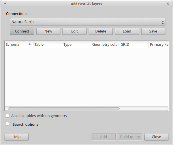
Start QGIS from the Desktop GIS menu and choose Add PostGIS layers from the layer menu. The
parameters for connecting to the OpenStreetMap data in PostGIS is already defined in the Connections
drop-down menu. You can define new server connections here, and store the settings for easy
recall. Click on Connections drop down menu and choose Natural Earth. Hit Edit if you want to see what those parameters are for Natural Earth, or just
hit Connect to continue:
You will now get a list of the spatial tables in the database:
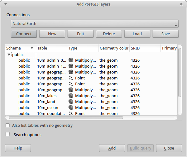
Choose the ne_10m_lakes table and hit Add at the bottom (not Load at the
top - that loads database connection parameters), and it should be
loaded into QGIS:
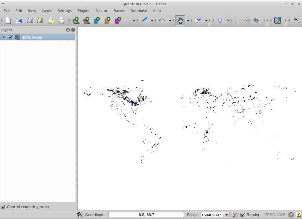
You should now see a map of the lakes. QGIS doesn’t know they are lakes, so might not colour them blue for you - use the QGIS documentation to work out how to change this. Zoom in to a famous group of lakes in Canada.
Creating A Spatial Table The Easy Way
Most of the OSGeo desktop tools have functions for importing spatial data in files, such as shapefiles, into PostGIS databases. Again we’ll use QGIS to show this.
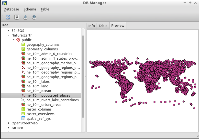
Importing shapefiles to QGIS can be done via the handy QGIS Database Manager. You find the manager in the menu. Go to Database -> DB Manager -> DB Manager.
Deploys the Postgis item, then the NaturalEarth item. It will then connect to the Natural Earth database. Leave the password blank if it asks. In the public item, there is the list of the layers provided by the database. You’ll see the main manager window. On the left you can select tables from the database and use the tabs on the right find out about them. The Preview tab will show you a little map.
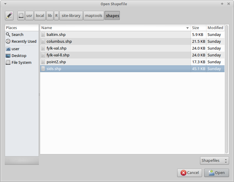
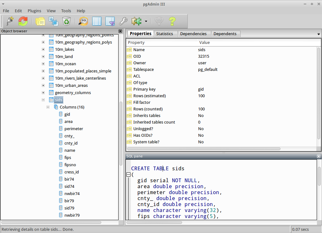
We will now use the DB Manager to import a shapefile into the database. We’ll use the North Carolina sudden infant death syndrome (SIDS) data that is included with one of the R statistics package add-ons.
From the Table menu choose the Import layer/file option.
Hit the ... button and browse to the sids.shp shapefile in the R maptools package
(located in /usr/lib/R/site-library/maptools/shapes/):
Leave everything else as it is and hit Load
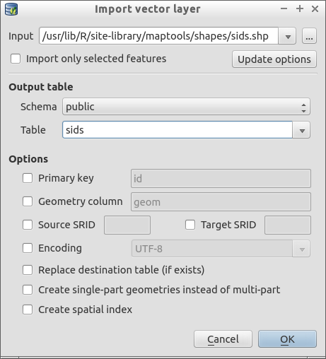
Let the Coordinate Reference System Selector default to (WGS 84 EPSG:4326) and hit OK. The shapefile should be imported into PostGIS with no errors. Close the PostGIS manager and
get back to the main QGIS window.
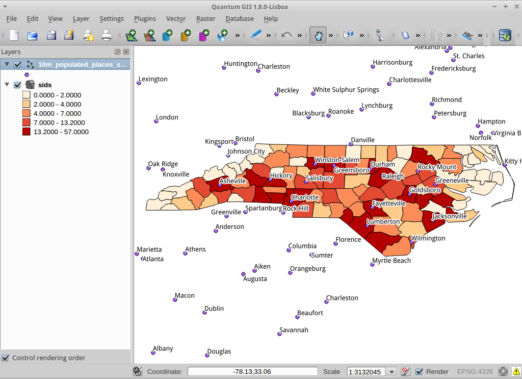
Now load the SIDS data into the map using the ‘Add PostGIS Layer’ option. With a bit of rearranging of the layers and some colouring, you should be able to produce a choropleth map of the sudden infant death syndrome counts in North Carolina:
Get to know pgAdmin III
You can use the graphical database client pgAdmin III from the Databases menu to query and modify your database non-spatially. This
is the official client for PostgreSQL, and lets you use SQL to manipulate your data tables. You can find and launch pgAdmin III
from the Databases folder, existing on the OSGeo Live Desktop.
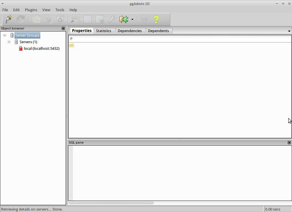
Here, you have the option of creating a new connection to a PostgreSQL server, or connecting to an existing server.
In this case, we are going to connect to the predefined local server.
After connection established, you can see the list of the databases already existing in the system.
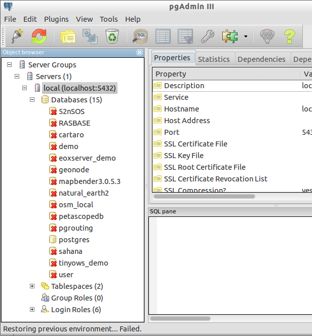
The red “X” on the image of most of the databases, denotes that you haven’t been yet connected to any of them (you are connected only
to the default postgres database).
At this point you are able only to see the existing databases on the system. You can connect, by double clicking,
on the name of a database. Do it for the natural_earth2 database.
You can see now that the red X disappeared and a “+” appeared on the left. By pressing it a tree is going to appear, displaying the contents of the database.
Navigate at the schemas subtree, expand it. Afterwards expand the
public schema. By navigating and expanding the
Tables, you can see all the tables contained within this schema.
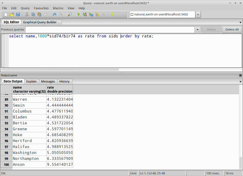
Executing a SQL Query from pgAdmin III
pgAdmin III, offers the capability of executing queries to a relational database.
To perform a query on the database, you have to press the SQL button from the main toolbar (the one with the
yellow Magnifying lens).
We are going to find the rate of the SIDS over the births for the 1974 for each city. Furthermore we are going to sort the result, based on the computed rate. To do that,we need to perform the following query (submit it on the text editor of the SQL Window):
select name, 1000*sid74/bir74 as rate from sids order by rate;
Afterwards, you should press the green arrow button, pointing to the right (execute query).
Things to try
Here are some additional challenges for you to try:
- Try some more spatial functions like
st_buffer(geom),st_transform(geom,25831),st_x(geom)- you will find full documentation at http://postgis.net/documentation/ - Export your tables to shapefiles with
pgsql2shpon the command line. - Try
ogr2ogron the command line to import/export data to your database. - Try to import data with
shp2pgsqlon the command line to your database. - Try to do road routing using
pgrouting_overview.
What Next?
This is only the first step on the road to using PostGIS. There is a lot more functionality you can try.
PostGIS Project home
PostGIS Documentation