

QGIS Quickstart
QGIS is a user friendly Desktop GIS client which lets you visualize, manage, edit, analyse data and compose printable maps.
Contents
Edit QGIS project
Let’s start by opening up an existing QGIS project, and turning layers on and off.
Launch QGIS from and select from the menu bar.
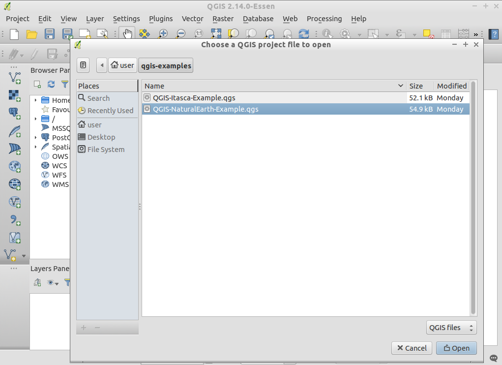
Choose
QGIS-NaturalEarth-Example.qgsand press Open.- You should see a world map.
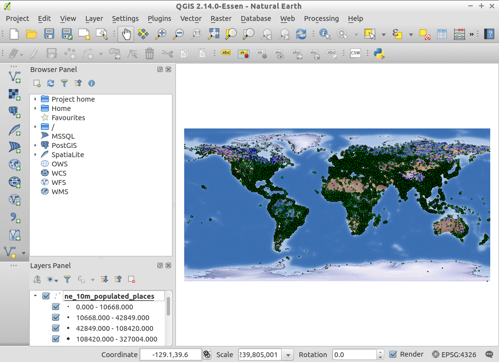
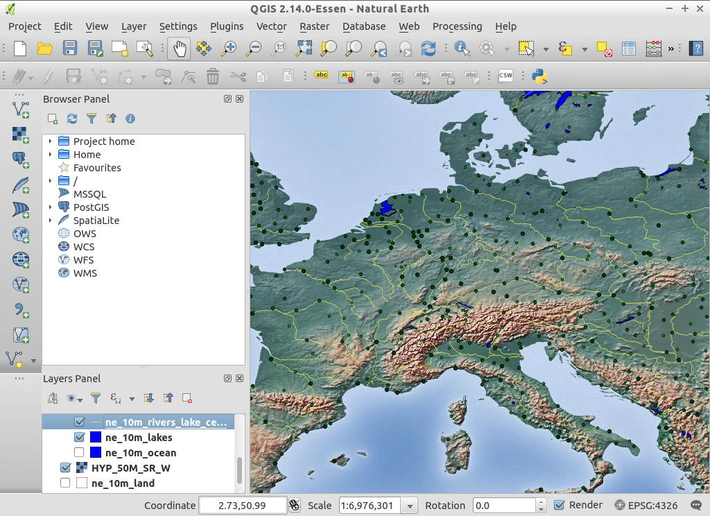
Tick the
ne_10m_populated_placescheck box in the Layers tree.Populated places are now displayed as many green dots:
Try dragging layers up and down in the legend and see how that affects visibility of the layers below.
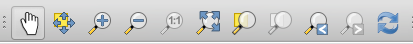
Have a look at the tools on the tool bar. Try panning, zooming in, and zooming back out to full extent again. Find these tools next to the hand icon. If the toolbars seem cluttered you can drag them around and turn them on and off by right clicking. You can also zoom in and out with the mouse wheel, and pan with a left-click drag.
Style a layer
Now let’s try customising the style of the map.
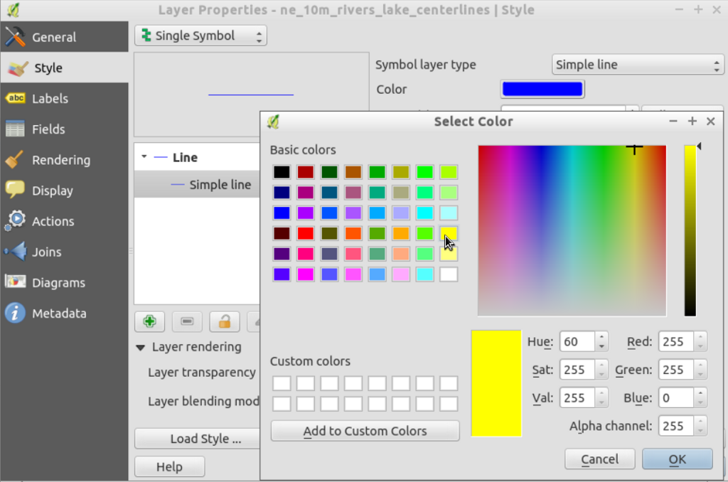
- Zoom in a little on the map, then double click
ne_10m_rivers_lake_centerlinesin the Layers tree.
#. In the Layer Properties dialog on the Style tab click on the Color to select a different color, say yellow.
Press OK.
Notice that rivers are now rendered in your new color.
Create a new QGIS project
Let’s now create a new QGIS project and load our own data.
- Choose . You will be asked whether to save the previous project, you can press Close without Saving.
#. Click Or click on the ‘Add Vector Layer’ button (the one with the ‘V’ shape, in the red rectangle in the image). You can also use the keyboard shortcut ‘Ctrl+Shift+V’
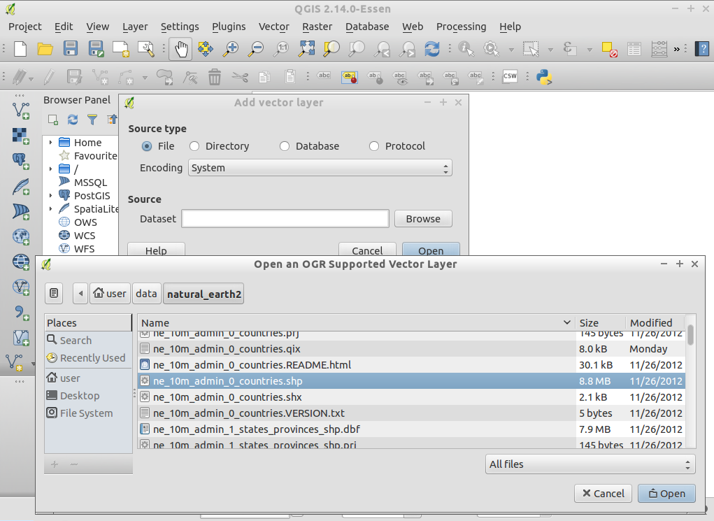
Browse to dataset
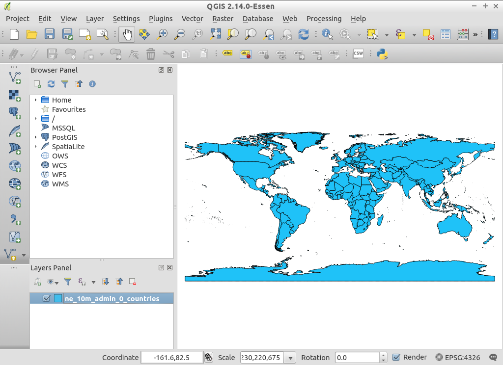
/home/user/data/natural_earth2/ne_10m_admin_0_countries.shp.Press Open then Open again.
You should see all world countries.
Connect to a PostGIS spatial database
Let’s now include a layer from a Postgres database.
- In the layer list on the left, untick the
ne_10m_admin_0_countriesvisibility check box to temporarily hide it. - Choose .
- You can also click on the icon with the elephant head in the left panel or use the keyboard shortcut ‘Ctrl+Shift+D’
- Both Natural Earth and OpenStreetMap Postgis databases are already available; we will be using use the Natural Earth database. If you wanted to connect to a different database, you would select the New button and fill in the database parameters.
#. Select the “Natural Earth” connection and press Connect. Then click on the Public schema to deploy it:
- A list of database tables will appear.
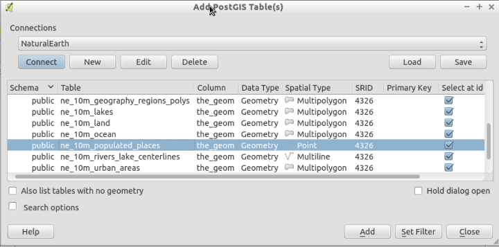
Select
ne_10_populated_placesand click Add.- For more details about working with PostGIS databases see the PostGIS Quickstart.
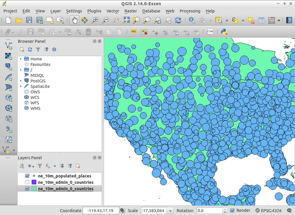
Zoom in on the United States using the mouse wheel and left-click drag to navigate.
Right click on
ne_10m_populated_placesin the layer list to get a context menu, then select .Let’s represent one of the database attributes in the data as a bubble plot. In the middle of the Style tab, drag the Transparency slider to 50%. Click on the small button at the right of the size field and select , then choose scalerank (it’s near to the beginning of the list). Then click Ok.
You can then click on the query button on the toolbar (cursor arrow with a blue “i”) and then on the map canvas bubbles to view information about the individual cities.
Using the GRASS Toolbox
There have been many plugins written for QGIS which extend QGIS’s core functionality. One of the more powerful is the GRASS plugin, which taps into the hundreds of geospatial processing modules available from GRASS GIS.
Note
You will need to change permissions of the grass data folder in order to carry out the following steps. Please open a terminal and execute the following: “sudo chmod -R 775 /usr/local/share/grass/nc_basic_spm_grass7”
Clear the slate with .
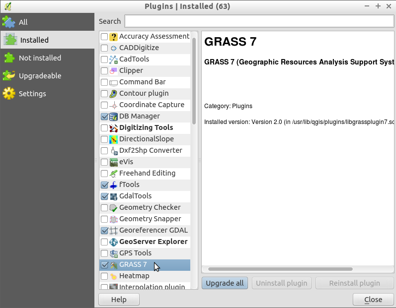
Choose , then scroll down or type
grassinto the Search box, and select the GRASS 7 plugin.- Notice that a new GRASS icon has been added to the Toolbar, a docked window named “GRASS Tools” has appeared on the right of the map area and a new GRASS menu item has been added to the Plugins menu.
Connect to an existing GRASS workspace with .
- The GRASS GIS data base (Gisdbase) has already been set to /home/user/grassdata on the disc for you.
Within the central GRASS data base are a number of sample datasets. We’ll load the North Carolina location, and the
user1mapset within it. Choose the nc_basic_spm_grass7 Location and user1 working mapset, then click Ok.To add a raster map to the QGIS layer list, navigate from QGIS Browser Panel to Home/grassdata/nc_basic_spm_grass7.
In the PERMANENT mapset select the elevation map and double click to add to the map.
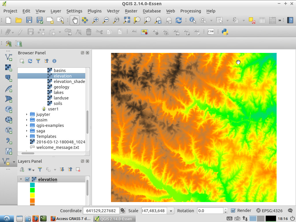
Add another GRASS raster layer, this time the geology map from the PERMANENT mapset.
- Double click on the geology map in the QGIS Layers list and in the Transparency tab set its global transparency to 70%.
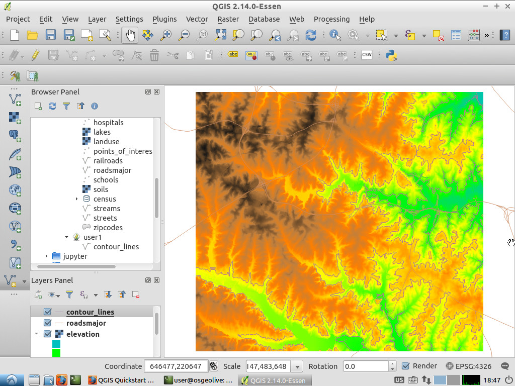
To add a vector map, select a vector layer from the QGIS Browser, similar to the previous steps.
- From the PERMANENT mapset select the roadsmajor map with a double click.
Change the layer order if neccessary (roadsmajor, geology, elevation).
The plugin also gives you access to many of the powerful GRASS analysis modules and visualization tools:
From the top menu select and drag the edge to make the window a bit bigger.
- A long list of analysis tools will appear. Go to the Modules Tree tab and
select .
Clicking on it will open a new tab. Select
elevationfrom the menu list and press Run. The elevation map will now have a thin red line around it, indicating the extent of GRASS’s computational region bounds.
- A long list of analysis tools will appear. Go to the Modules Tree tab and
select .
Clicking on it will open a new tab. Select
Back in the Modules Tree tab of the GRASS Tools window, go down to and select .
In the new module tab that pops open, select the elevation map as the input.
Add some contour levels (e.g. 20, 40, 60, 80, 100)
Select the output layer name (e.g. contour_lines), then click Run.
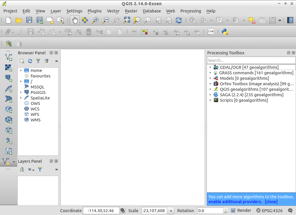
Using the Processing Toolbox
A core plugin for QGIS which opens the door to a large family of processing tools is the Processing Toolbox (formerly named the SEXTANTE Toolbox). It acts as a standardized wrapper around a number of other sets to tools.
Choose .
- A new toolbar will open on the right side of the screen with many processing tools to choose from. Take some time and have a look around.
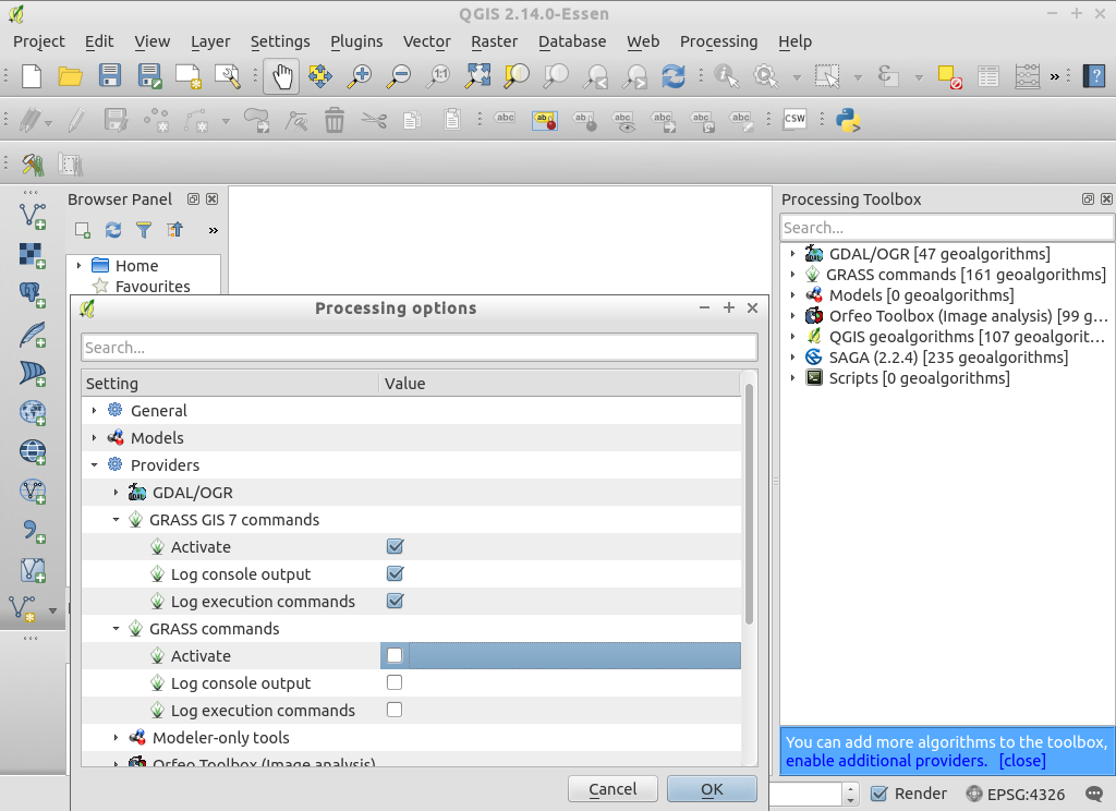
- You may need to enable a Processing provider in order to use it. The following screenshot shows how to enable GRASS GIS 7 support in the processing tools. Be sure to disable GRASS support (i.e., GRASS 6). Additionally, switch to the “Advanced Interface” (see lower right corner in the screenshot) in order to see the providers:
Importing OpenStreetMap data
Open the LX Terminal Emulator from the main menu.
Cut and paste the following commands into the Terminal window to create a working copy of the OSM data in the home directory:
cp data/osm/feature_city.osm.bz2 .
bzip2 -d feature_city.osm.bz2
In QGIS, choose . If you had the Processing Toolbox open you might want to close it.
Choose .
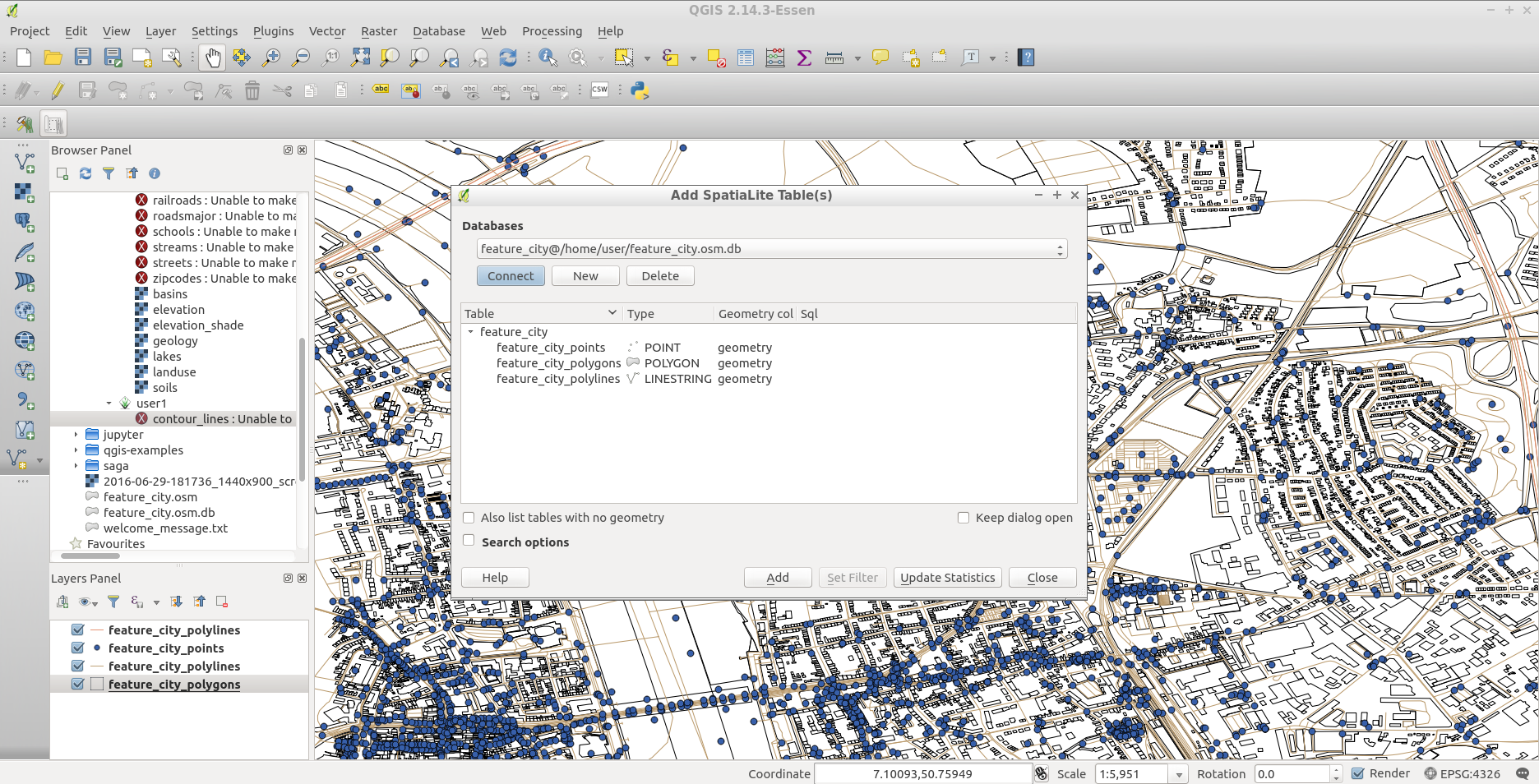
Click on the “…” button next to “Input XML file (.osm)” and select the feature_city.osm file you just copied into the home directory. The “Output SpatialLite DB file” name will be automatically set. Click Ok to convert the dataset to SpatiaLite format and create a connection to the SpatialLite DB within QGIS.
Next we need to extract points, lines, and areas, then add topology to each of these three new layers. To do this we need to run the tool three times. Select and use the “…” button to select the newly created feature_city.osm.db file. The Output layer name will be automatically filled in for you depending on the Export type selected. Click the Load from DB button to load in the available tags. For the “points” layer tick the amentity box; for the “polylines” layer tick the highway layer; and for the “polygon” layer select the building layer. You may wish to change the Output layer name to reflect the feature tags that you’ve selected. When you are ready, press Ok to load in the layer. You will need to again press the Load from DB button after changing the export type from points to polylines, and polylines to polygons.
Once topology is loaded, you can also refine the SpatiaLite layer by querying just certain features from within it. Select from the menu and from the Databases list select feature_city@… and then click on Connect. Double click on the feature_city_polylines table and then double click on “highway” to start building your SQL query. Then click on the = button, then the All button, and double click on motorway from the Values list. Click the Test button to verify the result, and finally click on Ok. Back in the Add SpatiaLite Table window click Add to restrict the rendering to just major highways. You can repeat this process with new layers to render different road types with different widths and styles.
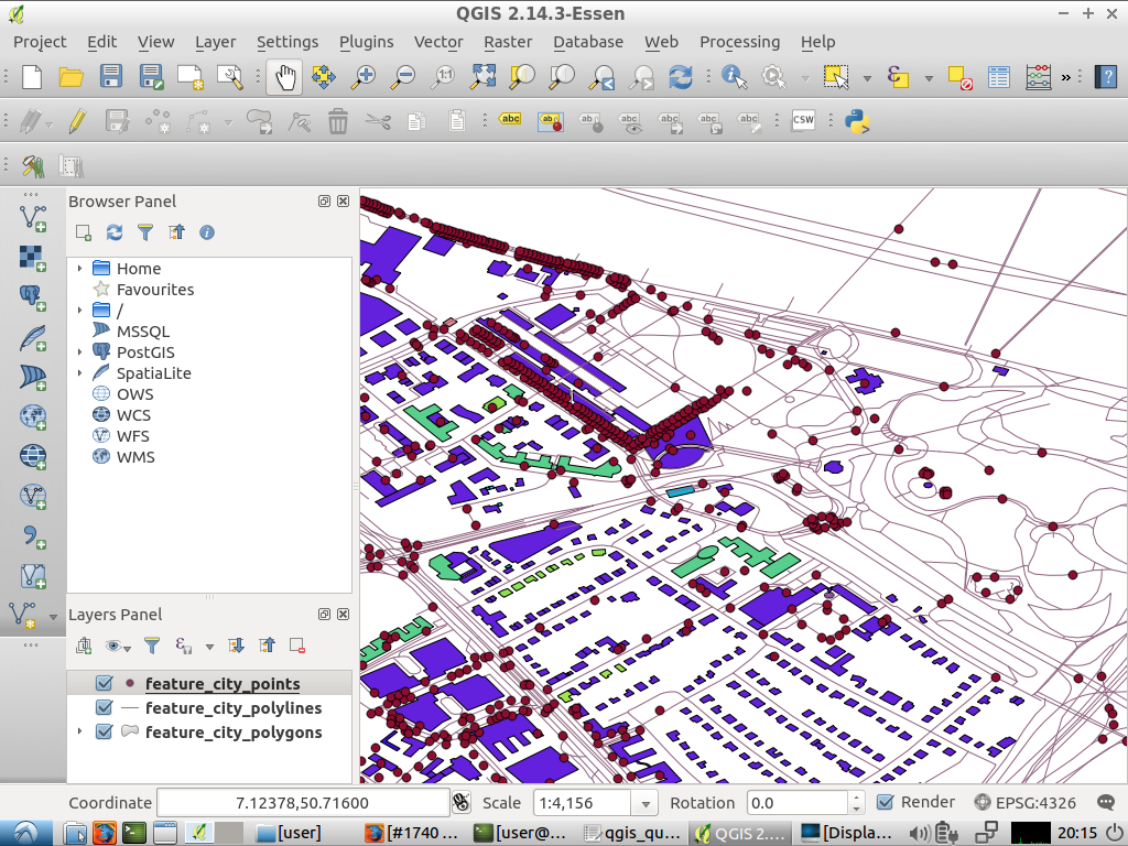
You can now explore this rich dataset. Use the
iinformation cursor button in the QGIS toolbar to query individal map features.
Things to Try
- Try viewing data sources with the QGIS Data Browser in the menu
- Try publishing your QGIS map to the web using QGIS Map Server in the menu.
What Next?
Tutorials for more advanced features of QGIS are collected as OSGeoLive QGIS tutorials.
To learn more about QGIS, a good starting point is the Documentation page on the QGIS homepage and A Gentle Introduction to GIS eBook.
The QGIS User Guide [1] is also included on the OSGeoLive disc.