../../_images/logo-gvSIG.png

gvSIG Quickstart

Project description

“gvSIG is a Geographic Information System (GIS), that is, a desktop application designed for capturing, storing, handling, analyzing and deploying any kind of referenced geographic information in order to solve complex management and planning problems. gvSIG is known for having a user-friendly interface, being able to access the most common formats, both vector and raster ones. It features a wide range of tools for working with geographic-like information (query tools, layout creation, geoprocessing, networks, etc.), which turns gvSIG into the ideal tool for users working in the land realm.” gvSIG 2011

This quickstart describes how to...

  • Start gvSIG and create a view;
  • Define the projection of a view;
  • Add raster and vector data to a view;
  • Navigate around a view;
  • Change how layers are presented in a view;
  • Select the towns that occur within a particular region and export these to a new file;
  • To create a map with a graticule; and
  • Save the current project or exit gvSIG.

Start gvSIG and create a view

Select gvSIG from the application menu. The application usually takes about a minute to startup.

  1. By default gvSIG opens with an empty project file with the ‘View’ document type selected.
  2. Click on the [New] button to create a view.
../../_images/gvsig_qs_0013.png

Define the projection of your view

Open the view properties dialog

  1. Select the newly created view. By default it is titled Untitled - 0 but may be Untitled - 1 if you created then deleted a view already.
  2. Click on the [Properties] button to open the View properties dialog.
  3. Click on the [...] button following the ‘Current projection’. This will open the New CRS dialog.
../../_images/gvsig_qs_0023.png

Defining your Coordinate Reference System

  1. Using the dropdown list for ‘Type’, select EPSG.
  2. Enter the EPSG code for the Coordinate Reference System. For this example we are using EPSG=4326, which is the WGS84 2D Geographic Projection. Then click on the [Search] button. This will list the selected CRS in the table below the search input field.
  3. Select [OK] to return to the View Properties dialog.
../../_images/gvsig_qs_0033.png

Saving the view properties

  1. Note that the EPSG code is now 4326 and that the map units have changed to degrees.
  2. Select [OK] to return to the Project Manager.
../../_images/gvsig_qs_0043.png

Open the view

  1. Select the newly created view.
  2. Click on the [Open] button to open the View.
  3. The view window consists of three zones.
  4. The top-left cell contains a list of vector or raster layers being used in the view (i.e. Table-of-Contents).
  5. The bottom-left cell displays the extent of the main view over a selected vector file.
  6. The right cell is the main display area where raster and vector data is rendered.
  7. Select the ‘Maximise window’ icon to have the view occupy the entire screen.
../../_images/gvsig_qs_0053.png

The View - adding raster and vector data

Open the add layer dialog

  1. Click on the ‘Add layer’ icon in the main toolbar to open the Add layer dialog.
  2. Select [Add] in the Add layer dialog. By default the first tab is File so the Open file dialog will appear.
  3. Drill down to the /usr/local/share/data/natural_earth/HYP_50M_SR_W directory.
../../_images/gvsig_qs_0063.png

Selecting a raster file

  1. Select gvSIG Raster Driver from the file type dropdown list. By default the shapefile driver is used so the directory may appear empty.
  2. Select HYP_50M_SR_W.tif.
  3. Click on the [OK] button to return to the Add layer dialog.
../../_images/gvsig_qs_0073.png

Selecting vector files

  1. The Add layer dialog now has the raster file listed.
  2. Select the [Add] button to add some vector files. The Open files dialog will appear.
  3. Select the [Up one level] button in the menu to change the directory to the /usr/local/share/data/natural_earth directory.
  4. Select gvSIG shp driver from the file type dropdown list.
  5. Select the 10m_admin_1_states_provinces.shp, 10m_populated_places_simple.shp and 10m_rivers_lake_centerlines.shp shapefiles from the list. Hold down the control key to select multiple files.
  6. Click on the [OK] button to return to the Add layer dialog.
  7. Click on the [OK] button on the Add layer dialog to return to the view.
../../_images/gvsig_qs_0083.png

The View - basic navigation

Zoom into a region

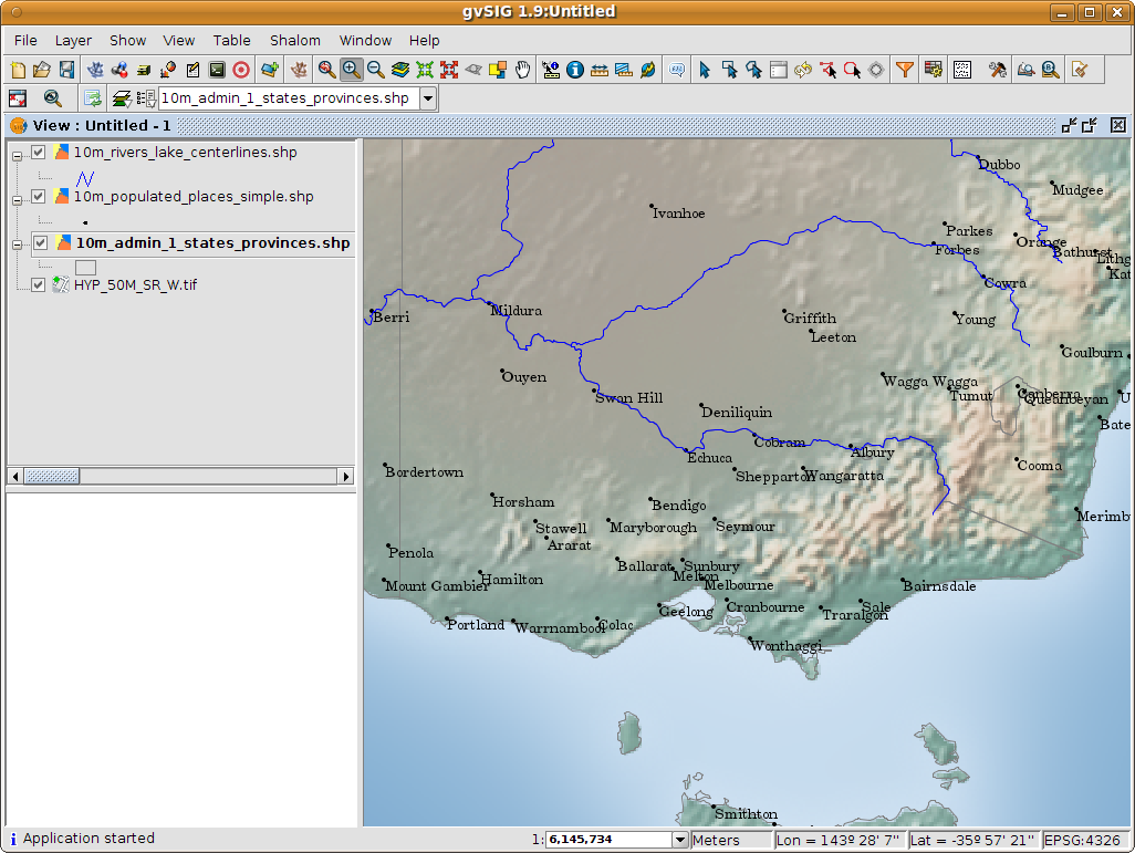
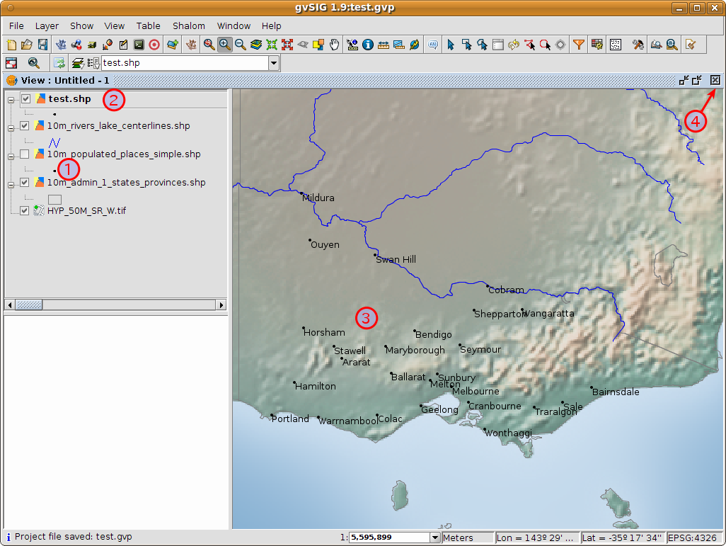
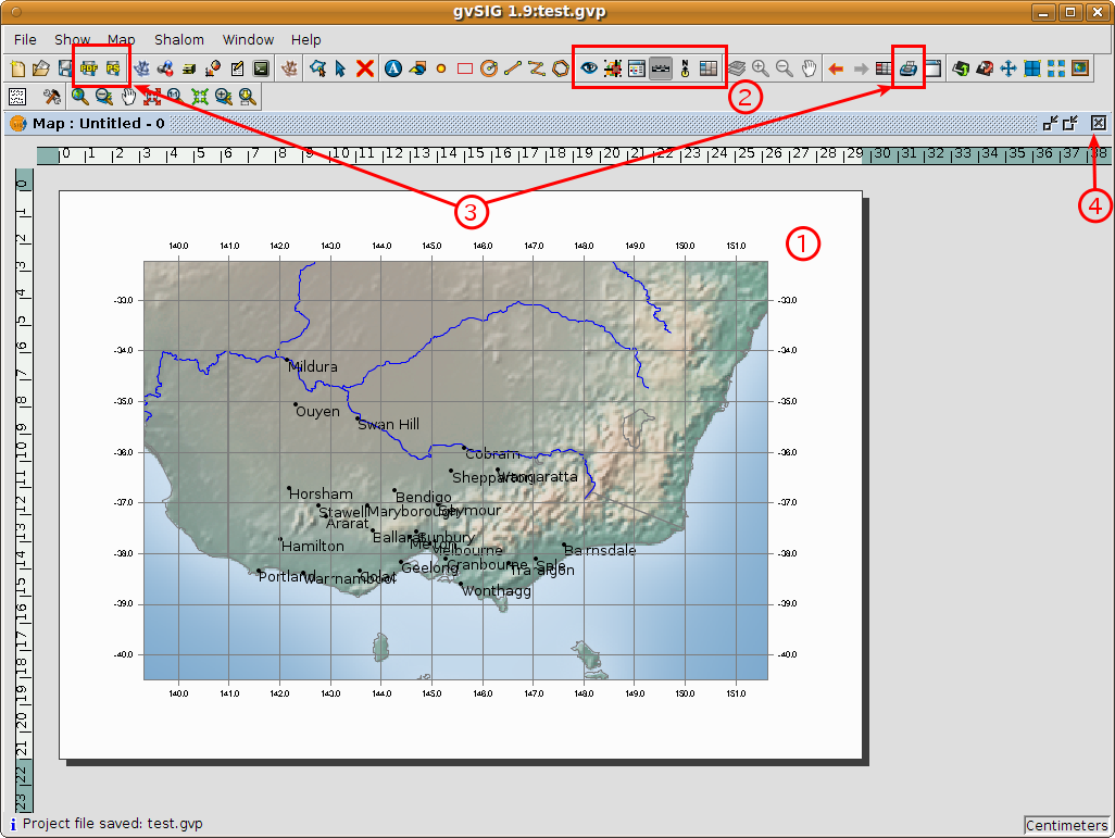
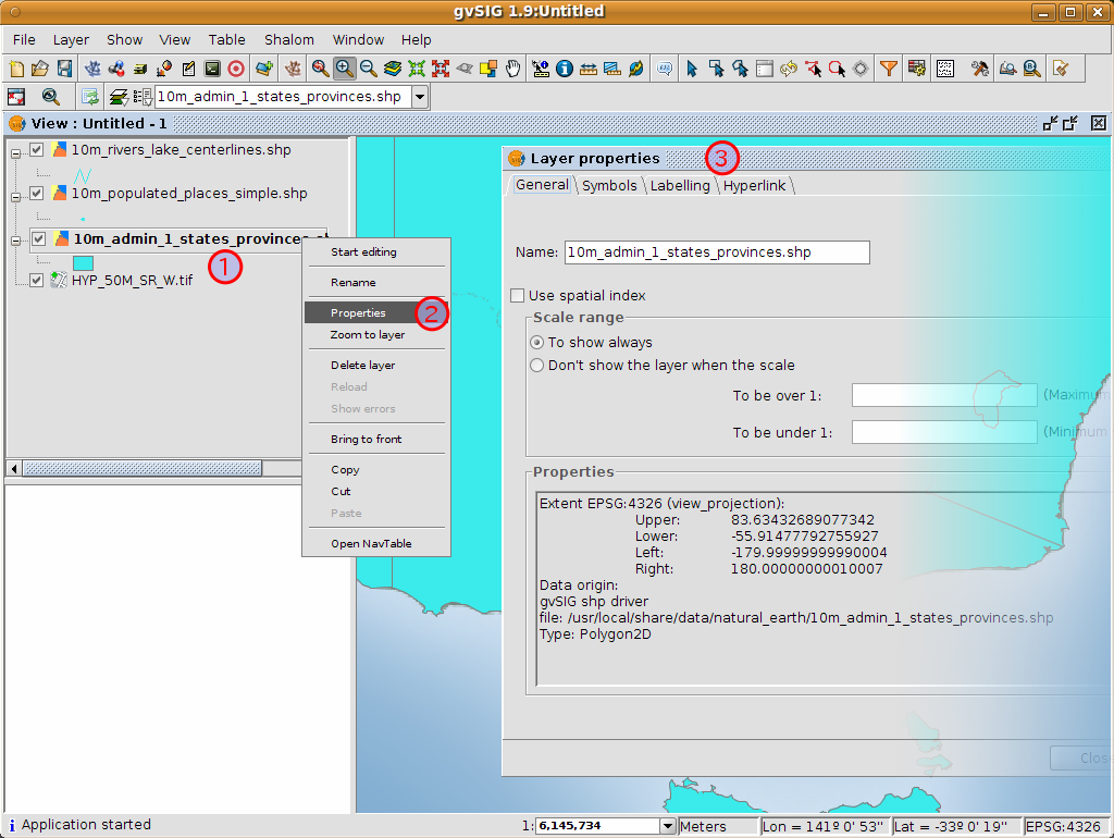
Once back at the main view you’ll see the vector files super-imposed over the raster file. The colours shown in this screen shot may differ from yours depending on the user preferences.

  1. By default the Zoom in tool is selected on the main toolbar.
  2. Use the mouse pointer to draw a bounding box around South-east Australia. Do this by selecting the top-left corner of the bounding box, holding down the left-mouse-button, and dragging the bottom-right corner of the bounding box over the selected area. Release the left-mouse button once you have the approximate area defined.
../../_images/gvsig_qs_0093.png

Fine-scale navigation

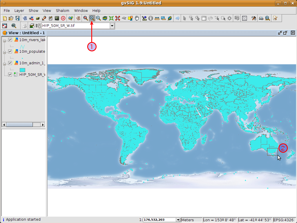
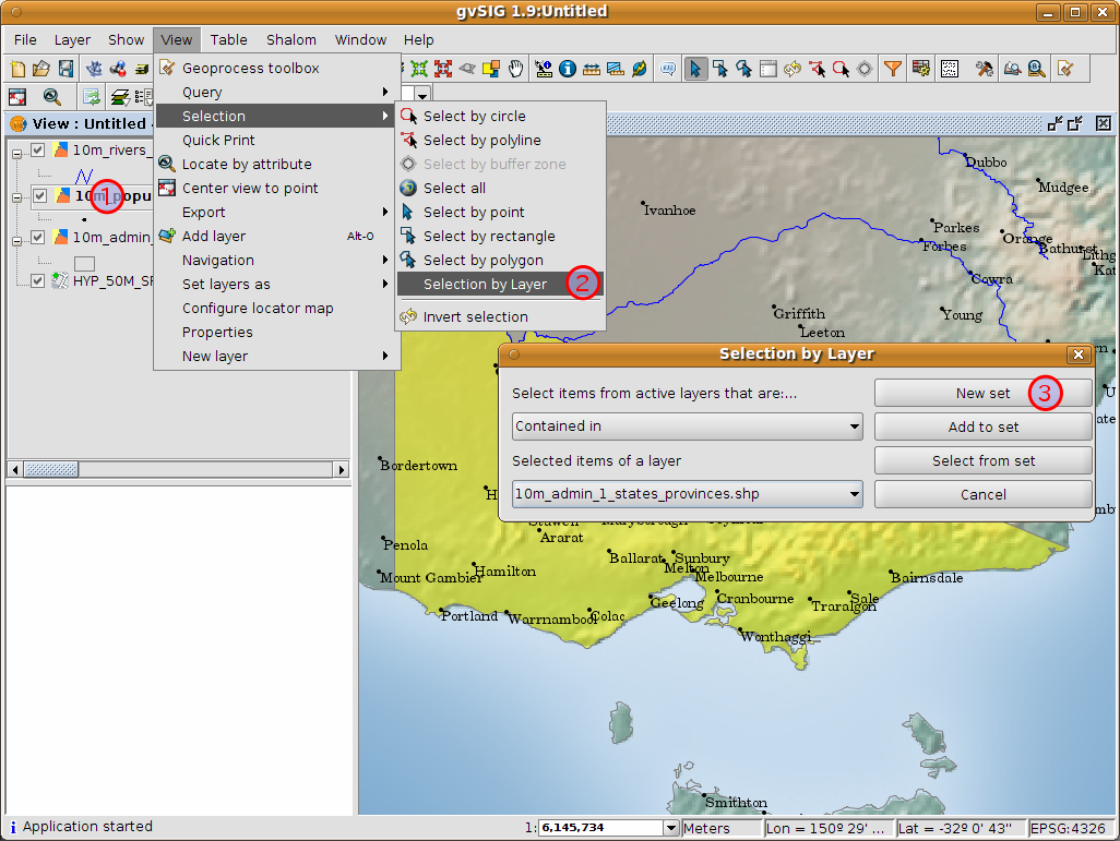
The view will automatically change to show the area within the selected bounding box.

  1. The size of the Table-of-Contents column can be adjusted using the mouse to help see long file names.
  2. Adjust what is shown in the view by using the highlighted tools, so that Victoria is central.
../../_images/gvsig_qs_0103.png

The View - changing how layers look

Making a polygon transparent

  1. Select the 10m_admin_1_states_provinces.shp layer using the left-mouse-button and click again with the right-mouse-button.
  2. Select the Properties submenu.
  3. The Layer properties dialog box will appear.
../../_images/gvsig_qs_0113.png

Changing the symbology of a vector layer

  1. Select the Symbols tab at the top of the Layers properties dialog.
  2. Select [Choose symbol] button so the Symbol selector dialog appears.
  3. Uncheck the Fill color box so the polygons are transparent.
  4. Click on the [OK] button to return to the Layers properties dialog.
../../_images/gvsig_qs_0123.png

Changing the labelling of a vector layer

  1. Select the Labelling tab at the top of the Layers properties dialog.
  2. Change the text attributes to those shown on the image, then click on the [Accept] button.
../../_images/gvsig_qs_0133.png

The result

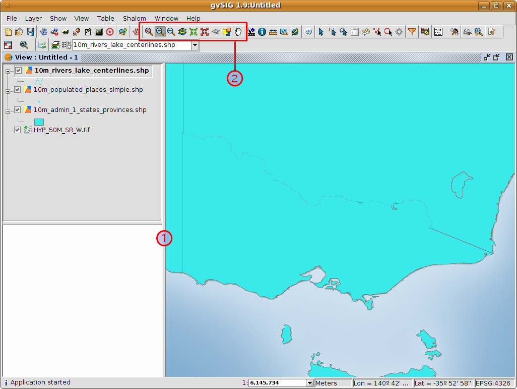
Note that this is a very basic view showing a point, a line and a polygon vector file superimposed over a raster file. It is just as easy to have an aerial photograph or Digital Terrain Model as a backdrop to your vector data, or to show other vector data stored in different formats.

../../_images/gvsig_qs_0143.png

A user exercise - change the symbology and labelling of the point and line layers

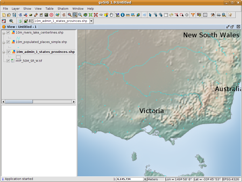
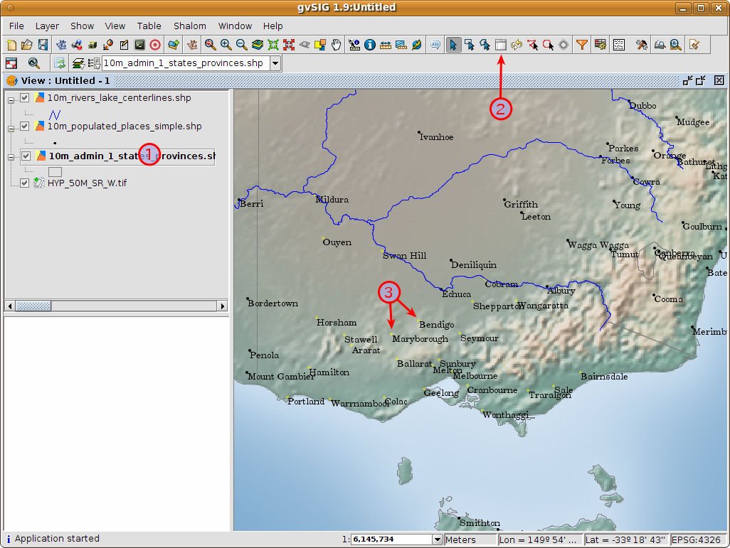
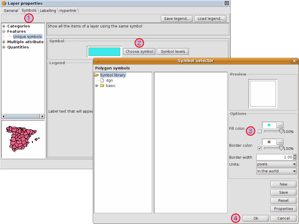
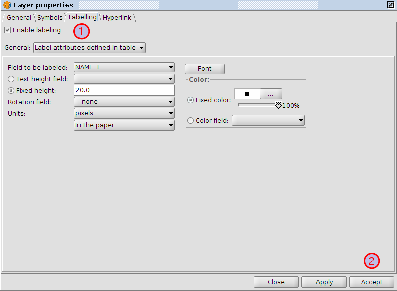
Following the previous few steps change the symbols, colour and labelling of the rivers and towns to generally match the following screen shot.

../../_images/gvsig_qs_0153.png

Simple analysis - select towns within a region

Selecting the region

  1. Select the 10m_admin_1_states_provinces.shp layer using the left-mouse-button.
  2. Select the ‘Select by point’ icon in the main toolbar.
  3. Click the polygon representing the State of Victoria. The polygon will go yellow or some other colour depending on your user preferences.
../../_images/gvsig_qs_0163.png

Selecting the towns contained within a region

  1. Select the 10m_populated_places_simple.shp layer using the left-mouse-button.
  2. Select View > Selection > Selection by layer to open the Selection by Layer dialog
  3. Change the two selection criteria using the dropdown boxes on the left-hand side of the Selection by Layer dialog. Click the [New set] button to select towns within the selected polygon.
  4. Select the [Cancel] button in the Selection by Layer dialog to return to the view.
../../_images/gvsig_qs_0173.png

Unselect the polygon so you can see what has happened

  1. Select the 10m_admin_1_states_provinces.shp layer using the left-mouse-button.
  2. Select the ‘Clear selection’ icon in the main toolbar.
  3. You can now see that the only those towns within Victoria are selected.
../../_images/gvsig_qs_0183.png

Export the selected towns to a new shapefile

  1. Select the 10m_populated_places_simple.shp layer using the left-mouse-button.
  2. Select Layer > Export to... > SHP to start the export.
  3. The Export to... dialog appears. gvSIG recognises that only 26 features are selected so warns you that only a subset of the shapefile will be exported. Select the [Yes] button to continue.
  4. The Save dialog appears. Give the file a name and save in a directory of choice. Select the [Save] button to continue. Note that if you already have a file by the name chosen a warning message will be shown.
  5. The Add layer dialog appears. Select the [Yes] button to add the new shapefile to the Table-of-Contents.
../../_images/gvsig_qs_0193.png

Showing only towns within a region

  1. Once you return to the view, uncheck 10m_populated_places_simple.shp in the Table-of-Contents.
  2. Change the symbology and labelling of test.shp to match the screenshot below.
  3. Now the view only includes towns and that occur within the State of Victoria.
  4. Select the ‘Close window’ icon to return to the Project manager so we can create a map using this view.
../../_images/gvsig_qs_0203.png

How to create a map

Create a new map and open it

  1. Select the Map document type in the Project Manager.
  2. Click on the [New] button to create a map.
  3. Select the newly created map. By default it is titled Untitled - 0.
  4. Click on the [Open] button.
  5. An empty map will appear in its own window titled Map: Untitled - 0. Note that a series of points are placed over the page. This is called a grid or guides and are used to snap elements to while formatting your map.
  6. Select the ‘Maximise window’ icon to have the map occupy the entire screen.
../../_images/gvsig_qs_0213.png

Insert a view with a grid/graticule

  1. Click on the ‘Insert view’ icon in the main menu
  2. Create a bounding box representing the extent of the map on the page by clicking on the empty map while holding down the left-mouse-button and dragging out the box, only letting go once the the area to be used is complete. This opens the Properties of view framework dialog.
  3. Select the view created earlier.
  4. Check the Show Grid option (this actually creates a graticule).
  5. Click on the [Configure] grid button to open the Grid settings dialog.
  6. In the Grid settings dialog change the grid interval to 1.0, that is 1 degree between lines representing latitude and longitude.
  7. Select the grid format (use lines rather than points for ease of viewing).
  8. Increase the font size to 14.
  9. Select the [Ok] button to return to the Properties of view framework dialog then select the [Accept] button to exit and return to your map.
../../_images/gvsig_qs_0223.png

What else can you do to a map?

  1. Select Map > Properties from the main menu to open the Map Properties dialog box. Unselect the Visualise Grid checkbox then select the [OK] button. The ‘snap-to’ guides/grid used while formatting should now be removed from the page and the image should match what is shown below.
  2. Additional elements like a scale and north arrow can be added to the map using the icons in the main toolbar or with the submenus in the Map menu.
  3. The map can be printed or exported to PDF or Postscript for incorporation into other works.
  4. Select the ‘Close window’ icon to return to the Project manager
../../_images/gvsig_qs_0233.png

Saving your project or exiting gvSIG

  1. Projects can be saved for use later by using the File > Save as... menu option, or
  2. Projects can be exited or closed by using the File > Exit menu option.
../../_images/gvsig_qs_0243.png

Where to from here...

Some English help and tutorials are available on the gvSIG website.

Copyright & Disclaimer