
This quickstart provides an introduction to a limited set of the functionality provided by MapWindow GIS v4.8.6 and it provides instructions on how to accomplish a suite of basic GIS tasks. My aim is to provide an easy-to-follow guide for users that are mainly interested in displaying GIS data, conducting simple queries, and exporting high quality maps for use in publications and presentations. This being the case, not all of the functionality of MapWindow is covered. In particular, the guide only covers the main program and not the plug-ins (except for the shapefile editor).
The MapWindow desktop software is available for free download as a single ready-to-install .exe file from the MapWindow website: www.mapwindow.org. MapWindow is a native Windows application that requires installation of the Microsoft .NET framework. It runs on XP, Vista, and Windows 7 and works fine on 64-bit machines. The program is quite intuitive to use and new users will be up and running quickly. With only a couple of exceptions it provides a user experience that meets or exceeds that of ArcMap, for the procedures covered in this guide.
The MapWindow desktop program that is the focus of this guide is just one part of a larger open-source project. The core software is also available as an ActiveX component, allowing programmers to develop customized GIS applications. It is also possible for advanced users to modify and extend the desktop program to fit individual needs. More information on the MapWindow project and its various facets can be obtained from the MapWindow website.
Because MapWindow is under continuous development it may not behave exactly as described in this guide if you are using a newer version of the program. A web-based users guide is under development in the MapWindow website and you might want to have a look there if you are running into problems or want information on functions not covered here.
The project file maintains a record of the different layers, labels, colors and styles you have defined for your map. When MapWindow starts it initiates a new project. You can also start a new project at any time by clicking the New toolbar button. Any changes that you make to a project are not stored until you click the Save toolbar button, or save when prompted on exit. Previous projects are accessed by clicking the Open toolbar button or selecting File from the top menu and clicking Recent Projects. You can also double click on the project file name in Windows Explorer, which opens the project in a new instance of MapWindow. Project files carry the extension .mwprj.
Besides saving the layers and related symbology the project file stores a few additional settings such as map units, projections, and so on. These can be accessed by selecting the File menu and clicking on Settings. Users will generally not have to make any changes to these settings so they will not be discussed here.
The installation program installs a number of core plug-ins, such Shapefile Editor, that provide additional functionality to the base program. Additional plug-ins are available from the MapWindow website. To install a new plug-in download the zip file and extract it to the MapWindow plug-in folder, usually C:\Program Files\MapWindow\Plugins. Sometimes the plug-in is a single .dll, but it can also be a folder containing multiple files in which case the whole folder goes into \MapWindow\Plugins.
Before you can use any of the plug-ins they have to be activated within MapWindow. To do this select Plug-ins from the main menu and click on the plug-in you wish to activate. It will remain activated, even in new projects, until you click it again. Once a plug-in is activated a new toolbar button or menu item will be displayed enabling you to use it.
The maps you produce will usually be composed of several GIS data layers. These layers are adding either by dragging and dropping files from Windows Explorer onto the map display window or by clicking the Add toolbar button. Each layer that is added is listed in the legend window (use View -> Panels -> Show Legend if it is not visible). Double clicking the layer in the legend or clicking the Properties toolbar button will bring up the Layer properties dialog which has several tabs for making changes to a layers properties. For example, to change the name displayed in the legend select the General tab and modify the text in the Name textbox. Other properties will be dealt with in subsequent sections. To remove a map layer click the Remove toolbar button. Clicking the Clear toolbar button will remove all map layers.
The colored icons displayed in the legend illustrate the type of data in the layers (polygon, line or point) and the current symbology. The order of the layers in the legend determines the overlay order in the map: layers that are higher in the list cover layers that are lower. If a layer seems to be missing it might be because it is completely covered by other layers. To change the order of a layer just click and drag it to where you want it to go. A small checkbox beside each legend entry allow you to turn the display of individual map layers on and off.
MapWindow will display different kinds of GIS data, including: vectors (polygons, lines, and points), rasters (rectangular grids of data), and images. Many different file formats are supported, including .shp, .asc, .aux, .bgd, .bil, .dem, dt1, .hdr, .img, .jpg, .sid, .std, .tif and others. The ESRI shapefile (.shp) is the vector format used by MapWindow when generating new vector files. It uses GeoTiff and the .bgd format when generating new raster files.
To add a scale to your map open the View menu and select Show Floating Scale Bar.
A projection is a mathematical transformation used to display the 3-dimensional earth onto your 2-dimensional computer screen. Different projections are available, each with its own benefits, costs, and appropriate uses. A detailed discussion of projections is beyond the scope of this guide, but a few basic points need to be covered. The main issue is that the various layers in your project all need to use the same projection if the overlays are to line up. In MapWindow, the projection of a layer is defined in a supplemental file carrying the .prj extension. This is a common format for projections, also used in ArcMap. A layers projection can be viewed in the General tab of the Layer Properties dialog, which is opened by double-clicking the layer in the legend or clicking the Properties toolbar button
The first map that you add to a project defines the projection for the entire project. Each subsequent layer must have the same projection or MapWindow will display a warning dialog. This dialog allows you to reproject the incoming layer, or do nothing (in which case the layers may be misaligned). Note that reprojecting a layer involves more than just changing the contents of the .prj file, there are also changes to the shape of the polygons. Therefore, it is best to reproject to a new file, rather than overwriting the old. If a map layer is missing the .prj file it will be necessary to define a projection for it. This can be done in MapWindow using the Toolbox, but the process is outside the scope of this guide.
A suite of basic map functions is accessed through a set of toolbar buttons. Their use is quite intuitive so only a brief explanation is provided here. Note that several functions require the user to first select a target layer, which is done by clicking it in the legend. You can move the toolbars (click and drag at the dotted line) and the text labels can be toggled on and off via right-click.

|
Zoom in: either click the area of interest or draw a bounding box. Zooming in and out can also be done using the mouse wheel. |

|
Zoom out. |

|
Zoom to the full extent of all visible layers. |

|
Zoom to selected shapes of the target layer. |

|
Move backwards through a list of earlier map views. |

|
Move forward through a list of earlier map views. |

|
Zoom to the extent of the target layer. |

|
Click and drag the map within the display window. |

|
Select shapes from the target layer. Ctrl-click to select multiple shapes, or draw a bounding box. See section 4.2 for more information on selections. |

|
Opens a dialog used to display the perimeter and area of shapes selected from the target layer or shapes drawn with the mouse. |

|
Click to view the attributes of shapes in the target layer. |
When you first add a layer all shapes are given the same color and outline. MapWindow has two dialogs for customizing the symbology (color scheme, outlines, style, etc.). One is the Layer Properties dialog, which can be accessed by double-clicking the layer in the legend.

The other is the Categories toolbar button. They both work much the same way. I will describe the Categories button here because I prefer using it.

If your layer is made of shapes that represent distinct entities, say herds of caribou, then proceed as follows. Click the Categories toolbar button to bring up the Symbology dialog. It will be empty when you begin, indicating that no symbology has been defined. Next, click the Generate Categories button (bottom left) to bring up the Category generation dialog. Follow the steps below to assign colors based on the attribute of your choice.
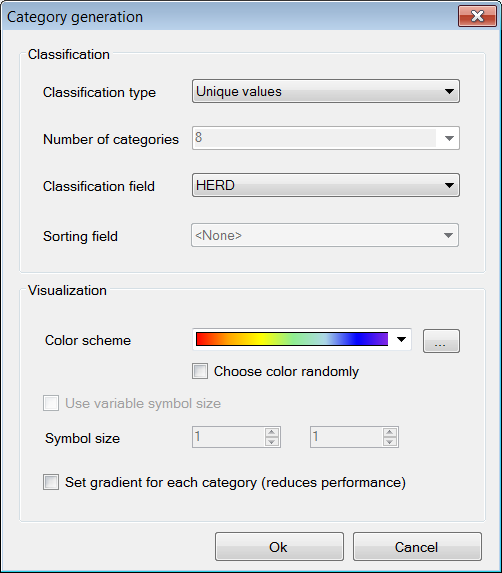
If your layer contains continuous data, say the height of trees within stands, then you must define categories into which the shapes are assigned. Begin by opening the Category generation dialog and selecting the classification field and color scheme as described in 3.1.1 Set the number of categories you want in the Number of categories box. Then, under Classification type select one of three methods for defining the category breakpoints: Equal intervals, Natural breaks, and Quantiles. These options will only be available if the classification field contains numeric data (use Unique values for text). Click Ok to complete the process.
If you wish to display the categories using a color ramp, say light red for low values grading to dark red for high values, select a smoothly grading color palette from the list of palette options (see example below). Do not check the Set gradient option because this refers to color gradients within polygons, something else entirely.
If your data layer is comprised of lines or points it may make more sense to illustrate gradients using symbol size (e.g., increasing line thickness or point size) rather than a color ramp. To do this place a check in the Use variable line width checkbox and then define the minimum and maximum symbol size in the option boxes below. Symbol size will be based on whatever attribute is selected in Classification field.
Once a color scheme has been generated, the categories and color assignments appear in the Shapefile categories dialog and in the legend. Further editing is possible from either location. For simple changes the fastest and easiest approach is to click on the color you want to change in the legend. But the dialog which opens with the Categories toolbar button has a few more options so I will focus on it here.
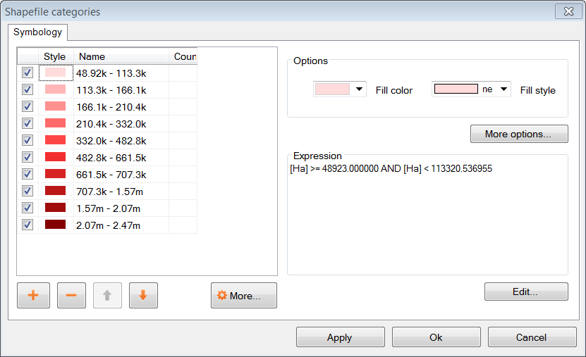
In the Shapefile categories dialog, select the category you wish to change by clicking on its name or color. Then:
Turn the display of the category on and off using the checkbox to the left of the name
Change the categorys name by typing over the existing text in the Name column (this only changes the legend entry; no changes are made to the attribute table)
Change the order that a category is listed in the legend using the up and down arrow buttons at the bottom of the dialog
Remove the category from the map by clicking the button with a minus sign
Set basic options for fill color and fill style using the option boxes in the top right corner of the dialog
Making the top layer partially transparent is a useful way of displaying features that lie beneath.
If you are working with continuous data you may want to fine-tune the category break points. For example, you may wish to flag all shapes that have a zero value with a unique color but display the rest of your data using a smooth color gradient. None of the classification schemes in the Category generation dialog will do this for you automatically. However, you can specify the breakpoints for each category manually using the Expression window of the dialog. The Expression window displays the current breakpoints in the form of a selection expression. Changing the breakpoints is simply a matter of typing new values into this expression and clicking Apply. It is up to you to ensure that your changes dont result in gaps between categories.
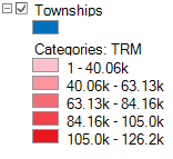
It is worth noting something here that can lead to unexpected results:when you generate categories, the original default symbology remains lurking in the background. In the example legend shown to the right a red color ramp has been assigned to the categories, but the original default color (blue) is still there too. Normally this is not an issue because all shapes are displayed using the category scheme. But if you manually define breakpoints and leave any gaps between categories the unassigned shapes will be seen in the default color. Another thing to keep in mind is that the default symbology is used as the template for generating categories. If you dont want your categories to have outlines, turn the outline off in the default symbology before generating the categories. Likewise, if you want the categories to have a fill, make sure it is visible in the default scheme first.
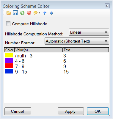
Raster layers use a different symbology dialog, called the Legend Editor, which is left over from an earlier version of MapWindow. To open the Legend Editor double-click on the layer in the legend. Scroll down to the Symbology section of the dialog and in the row labeled Coloring Scheme click Edit to bring up the Coloring Scheme Editor.
The buttons along the top of this dialog have basically the same functionality as the buttons along on the bottom of the Symbology dialog described in 3.1. The Generate categories button is called Wizard here, and takes the form of a yellow lightning bolt. It has a similar set of options and works in basically the same way. But only the Continuous Ramp option allows you to preselect your color scheme.
To change the color of a category just click on it in the Coloring Scheme Editor There is no option to display outlines for raster cells. The text that is displayed in the legend can be changed via the Text column and the breakpoint values can be manually changed via the Value column. Hillshade is outside of the scope of this guide.
Transparency is set in the Legend Editor, four rows down from Coloring Scheme. If a raster is sufficiently fine-scaled, transparency can be used to effectively combine information from the raster with other layers. To do this, move the raster to the top of the legend, assign a black to white color ramp, and set the transparency to about 50%. Whatever layer is beneath the raster will now be shaded according the rasters values. For example, a vector map of ecosystem types could be shaded on the basis of elevation, with lower elevations being darker and higher elevations being lighter.
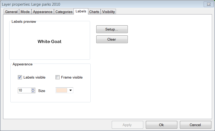
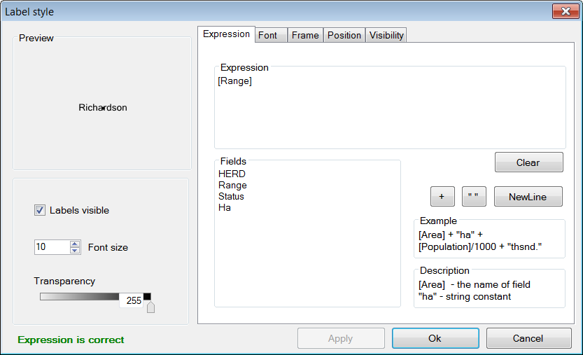
Labels are added using the Labels tab of the Layer Properties dialog, which is opened by double-clicking the layer in the legend. When you first open this dialog the label preview window will be empty. Click on the Setup button to proceed (see the screen shot on the next page). Clicking on the small label icon to the right of the layers name in the legend opens the same dialog. The Setup button brings up the Label Style dialog, defaulting to the Expression tab. The first step is to select the attribute that holds the label values. The available attributes are listed in the Fields window. Double-click on the appropriate attribute and it will show up in the Expression window, indicating that it has been selected. Click Apply and a pop-up will ask you how you want to anchor the labels.
Next, open the Font tab and select a font. Note that the default font may not be set, so you might not see anything until you assign the font here. Click Apply and the labels will appear on your map. The Label style dialog has many other options you can use to customize your labels, but none are mandatory. These options are fairly self-explanatory. Click Ok to finish.
Once labels have been generated you can change the text and style of individual entries by clicking on the Categories toolbar button. A new tab called Labels is now available (i.e., once labels have been defined). Initially it is empty, which means that all categories use the style you defined in Setup. To define unique styles for individual categories you must first generate label categories using the same approach as for generating symbology categories (Sec 3.1). Then use the rest of the dialog in the same way as described for the Shapefile categories dialog (see 3.1.3) to modify the appearance of individual category labels.

The positioning of labels can be fine-tuned using the Label Mover toolbar button. Just click and drag.

All symbology settings for a layer can be saved for use in future projects. This is done using the Symbology manager dialog, which is opened using the Symbology toolbar button. When you first open this dialog the preview window displays the symbology settings you have just defined. Click the Add Current button to save the current symbology. You will be prompted for a name. The file is saved in the same folder as the layer and carries an .mwsymb extension. If you make additional changes to the layers symbology you can save the new version under a new name. The dialog also has options for removing old symbology files and renaming them. Drag and drop adding of symbology files is not yet supported in MapWindow 4.8.6, but will be in a future version.
To apply a layers saved symbology in a new project, first add the layer to your map and then open the Symbology manager dialog. Previously saved symbology files will be listed in the Available options window. Select the one you want and click Apply options. Note that when you open a symbology file that includes labels, the labels may not be visible until you click Relabel shapefile, under the Layer menu.
You can also save the core symbology to a file (.mwleg) and then apply this symbology to other layers that have the same attribute structure (e.g., successive runs from a spatial model). Do this using the Save Categories and Load Categories options found under the More button at the bottom of the dialog that opens with the Categories toolbar button.
MapWindow provides two quick ways to export low-resolution maps. The first uses the Windows clipboard: open the View menu and select Copy. You can copy the map, legend, scale bar, and north arrow. In the second approach the same map components are exported to a file. Open the File menu and select Export. A wide variety of export file formats are available. For most maps the .png format will be best. When colors are uniform, as they typically are in maps, the .png format provides a high degree of compression without any changes to the image (i.e., lossless compression). To specify the export format just add the appropriate extension to your file name (e.g., Map1.png).
The low-resolution export described here is equivalent to a screen dump of the main map window. Note that the Preview Map, if you are using it, plays no role here. If there is a lot of white space in the main window, your exported map will have lots of white space. If you have minimized MapWindow (instead of running full screen), the map you produce will be small (basically a 1:1 ratio with what you see on the screen). The resolution of the map is equivalent to the resolution of your computer screen. This being the case, the exported maps are ok for use in PowerPoint but not for printing. Even though the map may look ok in Microsoft Word when its up on your screen, the image quality on paper will be poor.
Once you have your map looking the way you like it there are still a few steps required to prepare it for publication. As an example, say you are preparing a research paper or brochure and you want to add a map that will fit into a single column of text 7cm wide. The map you produce should have a resolution of 300 dpi (print quality) and fit into the allotted 7cm with a minimum of white space around it. It should also include an appropriate legend and perhaps a scale bar and north arrow. The Print Layout dialog, accessed under the File menu is intended to facilitate this process, but it is really just designed for printing, not publishing (i.e., the layout cannot be saved as a digital image). Also, the output resolution cannot be specified (just high and low), no modifications can be made to the legend, and there are limited options for defining a bounding box. This being the case, the best option (at present) for generating a publication quality map is to do some of the work in an image editor like Photoshop.
The first step in preparing your map for export is to define a bounding box for it. Do this by creating a simple rectangular shapefile that provides the margins you would like to see around your map (see 4.3). This layer must be included in your project, but it does not have to be visible. As an alternative you can use one of the existing layers in your project to define the map extent, but be aware that the output map will be tight-cropped (i.e., no margins). The practicality of defining a bounding box comes into play if you generate multiple maps with the same extent although margins can be added in Photoshop its tiring to have to do so for each and every map.
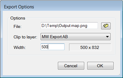
Next, open Export, under the File menu and select Georeferenced Map from the list of options. In the dialog that pops up enter a name for the map you are exporting in the File box. Remember to include the extension for the file type you want (e.g., .png). For Clip to layer select the layer that is to serve as your bounding box. If you havent defined a bounding box enter the layer with the largest extent. For Width, enter the desired width of your map in pixels. The value you enter here will depend on your desired resolution and your desired width. You will find that, in addition to your exported map, a second file with a .wld extension is generated during the export. This file can be deleted.
Export the legend, scale bar, and north arrow, as described in the previous section (3.5.1). Unfortunately, there is no way to generate high-resolution versions of these map elements in the current version of MapWindow. Frankly, I find the legend export to be of limited use anyway because there is no way to customize it (except for changing the layer names). Therefore, I generally produce my legend within Photoshop using a high resolution template I have made for this purpose. Producing a legend is simply a matter of adding the template to the base map, moving it to the right spot, changing the colors, and revising the text. It takes only a couple of minutes and produces a much better result than the cluttered low-resolution legend exported by MapWindow.
A word of caution. Many of the dialogs and processes discussed in this section can result in changes to your GIS data. MapWindow provides few warnings to alert you to such changes and the undo functionality is not yet working. Given the absence of a good safety net you should proceed carefully. For example, using Windows Explorer you might set the properties of important map layers to Read Only, or choose to work with copies instead of original maps.

Vector maps are linked to an attribute table that contains information for each shape. For example, if the shapes are forest stands the attribute table might include information on vegetation type, age, height, and so on. When you use the Identify toolbar button you are viewing information from the attribute table. To view the entire attribute table click the Table toolbar button, which brings up the Attribute Table Editor. This dialog allows you to view the data and also provides some basic database functionality. Some useful database functions provided by the table editor are summarized below.
| Function | Method |
|---|---|
| Modify a single data entry | Type over the existing data in a cell and it will be changed |
| Copy and paste individual data entries (there is no option for copying columns) | Right-click within a cell and select Copy or Paste |
| Add a new column | Edit -> Add field |
| Remove a column | Edit -> Remove field |
| Rename a column | Edit -> Rename field |
| Sort a column, ascending or descending | Right-click on the column title and select Sort Asc or Sort Desc |
| Summary statistics for a column | Right-click on the column title and select Statistics |
| Assign values to a column based on a mathematical expression | Right click on the column title and select Calculate values |
| Set an attribute to a constant value (for selected shapes only) | Right click on the column title and select Assign values |
| Generate a unique identifier for each shape | Tools -> Generate MWShapeID Field |
If changes have been made to the table a warning dialog will appear when the table editor is closed. Yes means commit the changes and No means discard the changes.
A feature that is missing in the current version of MapWindow is the ability to link external datasets to the attribute table (like Joins & Relates in ArcMap). Therefore, if you want to categorize and display shapes on the basis of an external attribute you must physically add the new attribute to the shapefiles attribute table. This can be done with a query in Microsoft Access or other database program. You can also use Excel, but unless you have an older version you will need to add a plug-in to Excel to provide support for .dbf export (.dbf is the file format that MapWindow and ArcMap use for the attribute table). A source for this plug-in is: http://es.sourceforge.jp/projects/sfnet_exceltodbf/ The merge can also be done using the Import External Data option of the Swift-D plug-in of MapWindow (though its slow). The attribute table editor has a tool called Generate MWShape ID field that can help you maintain the correct order in the table when you are merging external data.

Vector shapes can be selected in four ways:

(1) the select toolbar button, (2) the Query toolbar button, (3) the attribute table, and (4) the spatial query plug-in. The color used to highlight selected shapes can be changed in Appearance tab of the Layer Properties dialog. To clear a selection click Clear selection under the View menu. Selected shapes can be exported to a new shapefile using the ** selection** menu of the attribute table editor. Selections are also useful for visualizing queries and for limiting the scope of many geoprocessing procedures.
The ** select** button is used to manually select shapes. The target layer must first be selected in the legend. Click on a shape to select it. To add additional shapes hold Ctrl while clicking. If Ctrl is not held, then clicking a shape will cause any previous selections to be removed. In the current version of MapWindow there no way of unselecting individual shapes (all or none). To select a block of shapes click and draw a bounding box in the desired region.
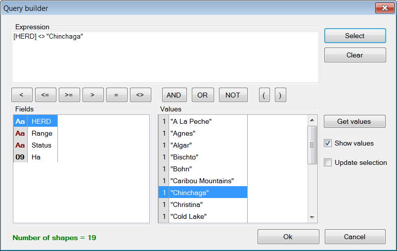
The Query button pulls up the Query builder dialog. This dialog is used to select shapes based on attributes defined in a search expression. The available attributes are listed in the Fields window. Double click the attribute you want and it will appear in the Expression window. Then select a logical symbol and the value you want to search for. When the expression is complete click ** select**. You are given the option of adding to an existing selection, excluding from an existing selection, or starting a new selection. The dialog will tell you how many shapes have been selected.
In the example shown on the previous page an expression was defined to search for all herds that do not have the name Chinchaga. A total of 19 shapes fit this description and were selected.

The attribute table can be used to both view and define selections. To view only selected shapes click the Show only selected shapes button, found in the toolbar near the top of the table editor. Click this button again to view all records. To select a record click the grey rectangle at the far left of the table. The record will be highlighted, indicating that it has been selected. Use the standard Windows shift-click to select multiple consecutive records, or just click and drag the mouse along the left. Use Ctrl-click to select multiple non-consecutive records. Clicking the Apply button is not required to make a selection.
Several important selection functions are found under the ** selection** menu, including: invert selection, select none, and select all. This menu is also where the option to export selected features is found. Export means create a new shapefile identical to the current layer but containing only the selected features. This is a useful way of producing derivative maps.
If the layer contains a large number of shapes it may be difficult to see a selected shape. You can zoom to the selected shape via the View menu or using the ** selected** toolbar button in the main MapWindow interface.
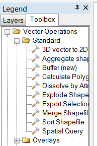
The Spatial Query dialog is a part of the GIS Toolbox, found under the legend. The path to the Spatial Query is: Legend -> Toolbox -> Vector Operations -> Standard.
A spatial query means selecting shapes from one layer based on their spatial relationship to shapes from another layer. For example, a query might select shapes from layer A if, and only if, they intersect with shapes from layer B. Several types of relationship can be specified, including: intersect, contain, touch, overlap, and others. It is possible to restrict the query to shapes in layer B that have been selected.
Shapefiles are added and modified using a plug-in called Shapefile Editor. Remember to activate the plug-in first in the Plug-ins menu. Doing so brings up a new toolbar that is used to run the plug-ins various functions. All references to toolbar buttons below refer to the shapefile editors toolbar. Note that this is a large toolbar and adding it can cause many of the other toolbars to be hidden. To avoid this you can grab the toolbar along the row of dots, and drag it down one row, or to wherever you want it.
A word of caution. The shapefile toolbar works on whatever layer happens to be selected in the legend. If you accidentally switch layers at some point there will be no warning to let you know that the target has changed. Furthermore, although the shapefile toolbar does have an Undo button, it is not yet functional in version 4.8.6. That said, you do have the option of setting the layer to Editing mode in the Mode tab of the Layer Properties dialog. This allows you to discard all changes when ending the editing session.
Shapefiles are created using the New toolbar button. Clicking New brings up a dialog in which you specify the name and location for the new file. You also select which type of shape you want: point, line, or polygon. Before creating a new shapefile you should load a layer into your project to set the projection and to serve as a spatial reference when adding your new shapes. Advanced techniques for georeferencing are beyond the scope of this guide.
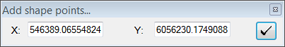
When a shapefile is created it is empty. To add freeform shapes use the Add toolbar button. There are two options for defining vertices. The easiest is to use the mouse each time you left-click a new vertex is added. When all the vertices have been defined, right-click the mouse to finish. An alternative approach is to define vertices by typing in their X and Y coordinates. A dialog is provided for this purpose when you click the Add button. After you have entered the X and Y values click the checkmark to the right to add the vertex. Then go on to the next, until you are done. Right-click to complete the shape and exit. Note that the X and Y boxes track the current location of the mouse, so dont let your mouse stray out of the dialog when entering the values or the values will be changed.
To add a regular shape (e.g., rectangle, circle, etc.) use the Insert toolbar button. First, pick the type of shape you want by clicking the Add this radio button of your choice. Next, fill in any required data (e.g., rectangle height and width). Then go to your map and click where you want the centroid of the new shape to be. Repeated clicking will produce multiple shapes. Once all of your shapes have been added click Done in the dialog to exit.
The shapefile toolbar has three buttons for changing the shape of existing shapes: Move vertex, Add vertex and Remove vertex. Vertices need not be visible to use these tools. When your mouse passes over an existing vertex it will be displayed, allowing you to move it (click and drag) or remove it (click) with the appropriate tool. If you are adding vertices, a new vertex will appear under your mouse when it travels near a shape (click to add). If the vertices are not immediately visible, wait a few seconds there is a slight lag when the tool initially loads. The shapes do not have to be selected for the tools to work. Until the Undo feature is functional it would be advisable to work with a copy of existing maps when modifying vertices, not the original, since the changes are committed immediately.
To remove shapes from a layer they must first be selected. Then click the Remove button to delete them. A warning box will pop up to ask you if you are sure.
Click the Merge button to merge individual shapes together. A dialog will pop up prompting you to select the shapes to be merged. The shapes to be merged must all belong to the same layer.
MapWindow includes a set of tools for common geoprocessing tasks. The main suite of tools is found in the GIS Toolbox, which is a tab under the legend. A few others exist as independent plug-ins. A description of geoprocessing operations is beyond the scope of this guide, but I will list some of the main operations here to provide readers with an understanding of the capabilities of MapWindow: