
To run GRASS on the Live DVD, click on the GRASS link on the desktop. From the “Welcome to GRASS” window select either the Spearfish or North Carolina (nc_spm_08) dataset for the location, and “user1” for the mapset, then click on [Start Grass].
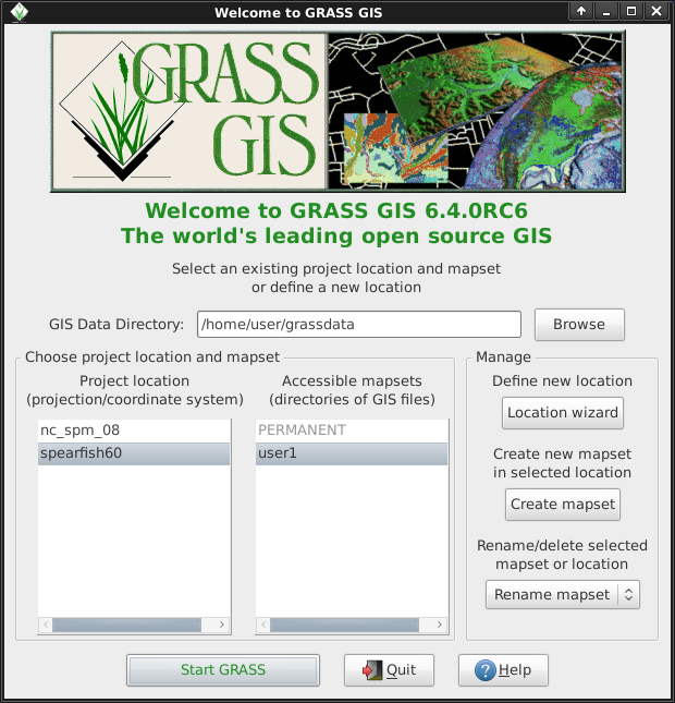
This will launch GRASS with our brand new GUI written in wxPython. At the time of writing we have gotten just about all of the kinks out of it and are nearly ready to call it (and GRASS 6.4.0) complete. The old Tcl/Tk GUI is still available if you prefer to use that; you can start it by typing g.gui --ui on the command line.
If you are on a netbook with a very small display (800x600 resolution) the startup screen might get a little scrunched and the [Start GRASS] button hidden behind the location and mapset lists. If this happens to you the solution is to drag the corner of the window to make it a little bigger. You might have to move the window up past the top of the screen a bit to get the room (hold down the Alt key and left-click drag the window to move it).
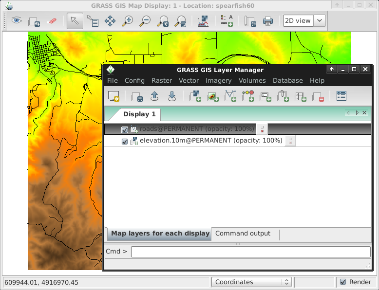
Once inside add a raster map layer such as “elevation” from the PERMANENT mapset. To do this go into the GIS Layer Manager window and click on the checkerboard toolbar button with a “+” on it. Then select the map name you want from the “map to be displayed” pull-down list, and click [Ok].
In a similar fashion add the “roads” vector layer from the PERMANENT mapset by clicking on the toolbar button with a “+” and a bent poly-line which looks a bit like a “V”.
Over in the Map Display window toolbar click on the eyeball button to render the view.
You should now see the maps displayed.
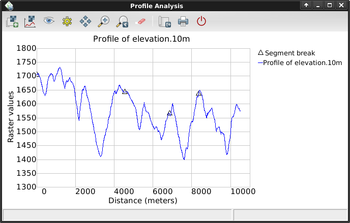
Back in the GIS Layer Manager window click on the elevation raster map name to select it. Then in the Map Display window, to the right of the zooming buttons on the Map Display toolbar is an icon with a line graph and checkerboard on it. Click on that and select Profile Surface Map. If it isn’t automatically listed again pick an elevation map as the raster layer and press [Ok]. The second button in from the left allows you to set out the profile line, click it then mark out a few points on the Map Display canvas. When done go back to the Profile window and click on the eyeball button to create the plot. Click on the I/O button of the far right to close the profile window.
Now let’s create a new map. Select Raster ‣ Generate surfaces ‣ Fractal surface from the menu (near the bottom); give your new map a name; adjust any options you like in the Options tab (the defaults are fine); and click [Run]. You can then [Close] the r.surf.fractal module’s dialog window.
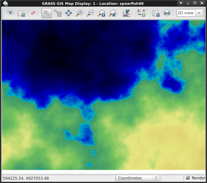
Now add your new raster layer to the layer list as you did before with the elevation raster map, except this time it will be in your “user1” working mapset. You might un-tick the elevation layer check-box now so that the two don’t draw over the top of each other. Click on the eyeball to view your new map. The colors might not be as you’d like so let’s change them. With the fractal DEM selected in the layer list, in the Raster menu select Manage colors ‣ Color Tables. In the “Colors” tab click on the pull-down list for the “Type of color table” option, and pick one from the list. “srtm” is a nice choice. Once done click the [Run] button and close the r.colors dialog window.
Because you have altered the map’s metadata, this time to re-render it you will have to fully flush the display cache. So click on the little refresh button next to the eyeball button to re-render all layers and you should see your map with its new colors.
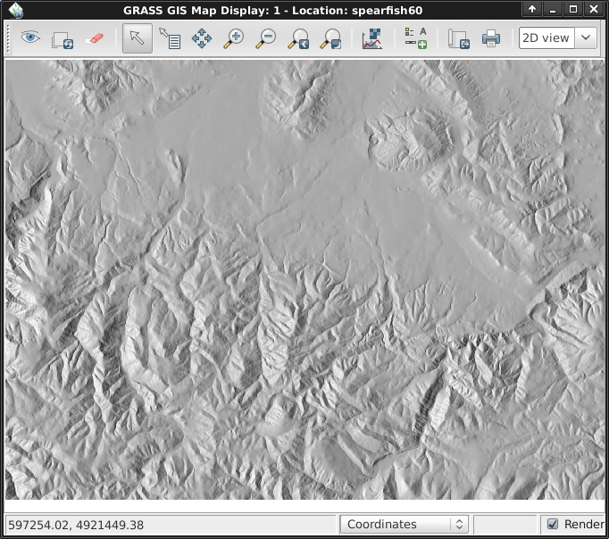
Next we’ll create a shaded relief map of the elevation layer we saw earlier. Start by verifying that the computational region is set match the raster map of interest, “elevation” in the PERMANENT mapset. To do this, make sure it is loaded into the layer list of the main Layer Manager window, right click on its name and select “Set computation region from selected map(s)”. In the Raster menu select Terrain analysis ‣ Shaded relief (Terrain analysis is about half way down), and the module control dialog will appear. With the elevation map name selected as the input map click [Run]. Now add the new elevation.shade @user1 map into your layer list and un-tick the other raster layers, then click the eyeball to re-render. (If you get sick of clicking the eyeball all the time you can tick the “Render” box in the bottom right of the Map Display window to have that happen automatically)
Once again select the elevation @PERMANENT map and in the Raster menu choose Hydrologic modeling ‣ Watershed analysis. This will open the r.watershed module. Set the elevation layer as your input map, in the ‘Input Options’ tab set the sub-basin threshold to 10000 cells, then in the ‘Output Options’ tab enter “elev.basins” for the watershed basin option and “elev.streams” for the stream segments option just below it. Then click [Run].
Back in the Layer Manager window add those two new raster maps to the layer list and make sure that they are the only two which are ticked for display in the box to the left of the layer name. Right click on the elev.basins raster map layer name and select “Change opacity level”. Set it to about 50% then re-render the Map Display.
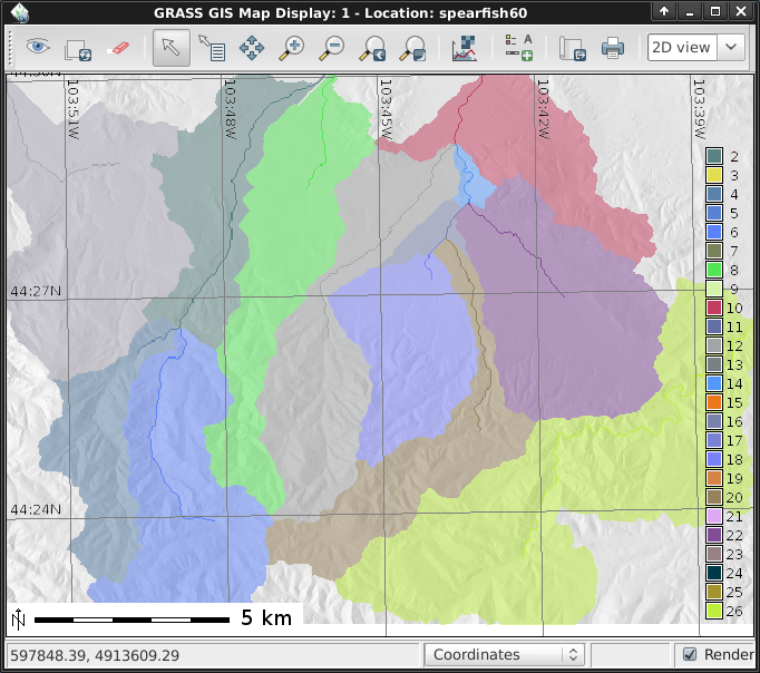
In the GIS Layer Manager window click on the third button in from the right to add a grid layer. For size of grid put 0:03 for 0 degrees and 3 minutes (format is D:M:S), then in the “Optional” tab tick Draw geographic grid and press [Run] and re-render.
To add a scalebar go to the Map Display window and press the “Add map elements” button to the right of where you selected the Profile tool earlier and select “Add scalebar and north arrow”. Read the instructions then click [Ok]. A scalebar will appear in the top left. Drag it down to the bottom left. From the same toolbar menu select “Add legend” and in the instructions window click the Set Options button to set the raster map name to create the legend for. After picking one click [Ok] and [Ok] again. Drag your new legend over to the right side of the map canvas.
Now you may be thinking to yourself that these fonts are a bit bare. That’s easily fixed in the GIS Layer Manager menus open Config ‣ Preferences and in the Display tab click the [Set font] button and then [Apply] in the Preferences window. You will have to do a full re-render to see the change so click on the re-render button next to the eyeball. The fonts will now be much prettier.
The above tasks have only covered a few raster modules. Don’t let this give you the idea that GRASS is just for raster maps – the vector engine and modules are every bit as full-featured as the raster ones. GRASS maintains a fully topological vector system which allows all sorts of very powerful analyses.
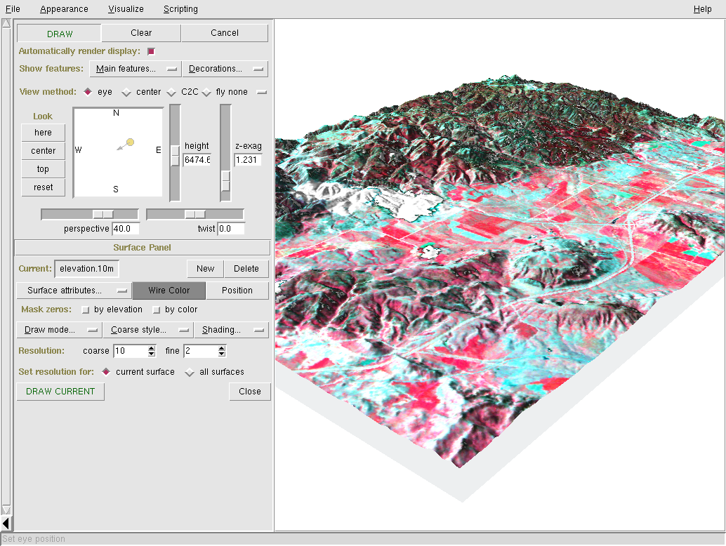
Start the 3D visualization suite from the File ‣ NVIZ menu item. Select an elevation map as the raster elevation. Once the 3D display interface loads, maximize the window. Next select Visualize ‣ Raster Surfaces from the top menu, and set the fine resolution to “1”, then move the positioning puck and height slider around to get different views.
To drape satellite or aerial imagery over the top of the DEM, in the Raster Surfaces controls click on the Surface Attributes drop down menu and select “color”. Select “New Map” to pick the overlay image. In the Spearfish dataset “spot.image” in PERMANENT is a good choice; in the North Carolina dataset “lsat7_2002_50” in PERMANENT is a good choice. Finally, click “Accept” and then once back at the main window click on the “Draw” button in the top-left, just under the File menu.
When finished, exit the GRASS GUI with File ‣ Exit. Before you close the GRASS terminal session as well, try a GRASS module by typing “g.manual --help” which will give you a list of module options. The GRASS command line is where the true power of the GIS comes into its own. GRASS is designed to allow all commands to be tied together in scripts for large bulk processing jobs. Popular scripting languages are Bourne Shell and Python, and some neat tricks for making scripting easier are included for both. With these tools you can make a new GRASS module with only about 5 minutes of coding, complete with powerful parser, GUI, and help page template.
“g.manual -i” will launch a web browser with the module help pages. When done close the browser and type “exit” at the GRASS terminal prompt to leave the GIS environment.